In “Discretization of a Schrödinger Hamiltonian” we have learnt that Kwant works
with tight-binding Hamiltonians. Often, however, one will start with a
continuum model and will subsequently need to discretize it to arrive at a
tight-binding model.
Although discretizing a Hamiltonian is usually a simple
process, it is tedious and repetitive. The situation is further exacerbated
when one introduces additional on-site degrees of freedom, and tracking all
the necessary terms becomes a chore.
The continuum sub-package aims to be a solution to this problem.
It is a collection of tools for working with
continuum models and for discretizing them into tight-binding models.
See also
The complete source code of this tutorial can be found in
discretize.py
As an example, let us consider the following continuum Schrödinger equation for a semiconducting heterostructure (using the effective mass approximation):
Replacing the momenta by their corresponding differential operators
for \(\alpha = x, y\) or \(z\), and discretizing on a regular lattice of points with spacing \(a\), we obtain the tight-binding model
with \(A(x) = \frac{\hbar^2}{2 m(x)}\).
discretize to obtain a template¶The function kwant.continuum.discretize takes a symbolic Hamiltonian and
turns it into a Builder instance with appropriate spatial
symmetry that serves as a template.
(We will see how to use the template to build systems with a particular
shape later).
    template = kwant.continuum.discretize('k_x * A(x) * k_x')
    print(template)
It is worth noting that discretize treats k_x and x as
non-commuting operators, and so their order is preserved during the
discretization process.
The builder produced by discretize may be printed to show the source code of its onsite and hopping functions (this is a special feature of builders returned by discretize):
# Discrete coordinates: x

# Onsite element:
def A(site, A):
    (x, ) = 1 * site.tag
    _const_0 = (A(1/2 + x))
    _const_1 = (A(-1/2 + x))
    return (_const_0 + _const_1)

# Hopping from (1,):
def A(site1, site2, A):
    (x, ) = 1 * site1.tag
    _const_0 = (A(1/2 + x))
    return (-_const_0)
kwant.continuum uses sympy internally to handle symbolic
expressions. Strings are converted using kwant.continuum.sympify,
which essentially applies some Kwant-specific rules (such as treating
k_x and x as non-commutative) before calling sympy.sympify
The builder returned by discretize will have an N-D
translational symmetry, where N is the number of dimensions that were
discretized. This is the case, even if there are expressions in the input
(e.g. V(x, y)) which in principle may not have this symmetry. When
using the returned builder directly, or when using it as a template to
construct systems with different/lower symmetry, it is important to
ensure that any functional parameters passed to the system respect the
symmetry of the system. Kwant provides no consistency check for this.
The discretization process consists of taking input \(H(k_x, k_y, k_z)\), multiplying it from the right by \(\psi(x, y, z)\) and iteratively applying a second-order accurate central derivative approximation for every \(k_\alpha=-i\partial_\alpha\):
This process is done separately for every summand in Hamiltonian.
Once all symbols denoting operators are applied internal algorithm is
calculating gcd for hoppings coming from each summand in order to
find best possible approximation. Please see source code for details.
Instead of using discretize one can use
discretize_symbolic to obtain symbolic output.
When working interactively in Jupyter notebooks
it can be useful to use this to see a symbolic representation of
the discretized Hamiltonian. This works best when combined with sympy
Pretty Printing.
The symbolic result of discretization obtained with
discretize_symbolic can be converted into a
builder using build_discretized.
This can be useful if one wants to alter the tight-binding Hamiltonian
before building the system.
Let us now use the output of discretize as a template to
build a system and plot some of its energy eigenstate. For this example the
Hamiltonian will be
where \(V(x, y)\) is some arbitrary potential.
First, use discretize to obtain a
builder that we will use as a template:
    hamiltonian = "k_x**2 + k_y**2 + V(x, y)"
    template = kwant.continuum.discretize(hamiltonian)
    print(template)
We now use this system with the fill
method of Builder to construct the system we
want to investigate:
    def stadium(site):
        (x, y) = site.pos
        x = max(abs(x) - 20, 0)
        return x**2 + y**2 < 30**2

    syst = kwant.Builder()
    syst.fill(template, stadium, (0, 0));
    syst = syst.finalized()
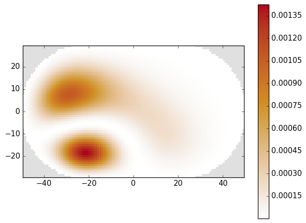
After finalizing this system, we can plot one of the system’s energy eigenstates:
def plot_eigenstate(syst, n=2, Vx=.0003, Vy=.0005):

    def potential(x, y):
        return Vx * x + Vy * y

    ham = syst.hamiltonian_submatrix(params=dict(V=potential), sparse=True)
    evecs = scipy.sparse.linalg.eigsh(ham, k=10, which='SM')[1]
    kwant.plotter.map(syst, abs(evecs[:, n])**2, show=False)
Note in the above that we provided the function V to
syst.hamiltonian_submatrix using params=dict(V=potential), rather than
via args.
In addition, the function passed as V expects two input parameters x
and y, the same as in the initial continuum Hamiltonian.
When working with multi-band systems, like the Bernevig-Hughes-Zhang (BHZ)
model [1] [2], one can provide matrix input to discretize
using identity and kron. For example, the definition of the BHZ model can be
written succinctly as:
    hamiltonian = """
       + C * identity(4) + M * kron(sigma_0, sigma_z)
       - B * (k_x**2 + k_y**2) * kron(sigma_0, sigma_z)
       - D * (k_x**2 + k_y**2) * kron(sigma_0, sigma_0)
       + A * k_x * kron(sigma_z, sigma_x)
       - A * k_y * kron(sigma_0, sigma_y)
    """

    template = kwant.continuum.discretize(hamiltonian, grid_spacing=a)
We can then make a ribbon out of this template system:
    def shape(site):
        (x, y) = site.pos
        return (0 <= y < W and 0 <= x < L)

    def lead_shape(site):
        (x, y) = site.pos
        return (0 <= y < W)

    syst = kwant.Builder()
    syst.fill(template, shape, (0, 0))

    lead = kwant.Builder(kwant.TranslationalSymmetry([-a, 0]))
    lead.fill(template, lead_shape, (0, 0))

    syst.attach_lead(lead)
    syst.attach_lead(lead.reversed())

    syst = syst.finalized()
and plot its dispersion using kwant.plotter.bands:
    kwant.plotter.bands(syst.leads[0], params=params,
                        momenta=np.linspace(-0.3, 0.3, 201), show=False)
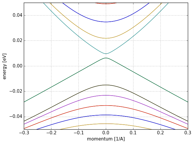
In the above we see the edge states of the quantum spin Hall effect, which
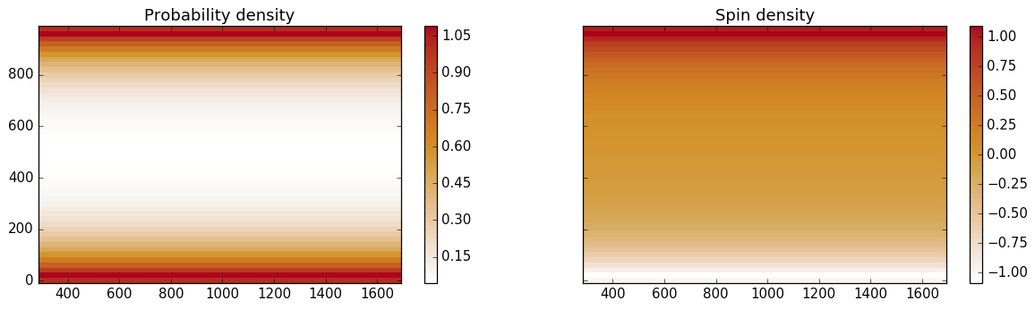
we can visualize using kwant.plotter.map:
    # get scattering wave functions at E=0
    wf = kwant.wave_function(syst, energy=0, params=params)

    # prepare density operators
    sigma_z = np.array([[1, 0], [0, -1]])
    prob_density = kwant.operator.Density(syst, np.eye(4))
    spin_density = kwant.operator.Density(syst, np.kron(sigma_z, np.eye(2)))

    # calculate expectation values and plot them
    wf_sqr = sum(prob_density(psi) for psi in wf(0))  # states from left lead
    rho_sz = sum(spin_density(psi) for psi in wf(0))  # states from left lead

    fig, (ax1, ax2) = plt.subplots(1, 2, sharey=True, figsize=(16, 4))
    kwant.plotter.map(syst, wf_sqr, ax=ax1)
    kwant.plotter.map(syst, rho_sz, ax=ax2)
It is important to remember that the discretization of a continuum model is an approximation that is only valid in the low-energy limit. For example, the quadratic continuum Hamiltonian
and its discretized approximation
where \(t=\frac{\hbar^2}{2ma^2}\), are only valid in the limit \(E < t\). The grid spacing \(a\) must be chosen according to how high in energy you need your tight-binding model to be valid.
It is possible to set \(a\) through the grid_spacing parameter
to discretize, as we will illustrate in the following
example. Let us start from the continuum Hamiltonian
We start by defining this model as a string and setting the value of the \(α\) parameter:
    hamiltonian = "k_x**2 * identity(2) + alpha * k_x * sigma_y"
    params = dict(alpha=.5)
Now we can use kwant.continuum.lambdify to obtain a function that computes
\(H(k)\):
        h_k = kwant.continuum.lambdify(hamiltonian, locals=params)
        k_cont = np.linspace(-4, 4, 201)
        e_cont = [scipy.linalg.eigvalsh(h_k(k_x=ki)) for ki in k_cont]
We can also construct a discretized approximation using
kwant.continuum.discretize, in a similar manner to previous examples:
        template = kwant.continuum.discretize(hamiltonian, grid_spacing=a)
        syst = kwant.wraparound.wraparound(template).finalized()

        def h_k(k_x):
            p = dict(k_x=k_x, **params)
            return syst.hamiltonian_submatrix(params=p)

        k_tb = np.linspace(-np.pi/a, np.pi/a, 201)
        e_tb = [scipy.linalg.eigvalsh(h_k(k_x=a*ki)) for ki in k_tb]
Below we can see the continuum and tight-binding dispersions for two different values of the discretization grid spacing \(a\):
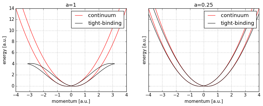
We clearly see that the smaller grid spacing is, the better we approximate the original continuous dispersion. It is also worth remembering that the Brillouin zone also scales with grid spacing: \([-\frac{\pi}{a}, \frac{\pi}{a}]\).
The input to kwant.continuum.discretize and kwant.continuum.lambdify can be
not only a string, as we saw above, but also a sympy expression or
a sympy matrix.
This functionality will probably be mostly useful to people who
are already experienced with sympy.
It is possible to use identity (for identity matrix), kron (for Kronecker product), as well as Pauli matrices sigma_0,
sigma_x, sigma_y, sigma_z in the input to
lambdify and discretize, in order to simplify
expressions involving matrices. Matrices can also be provided explicitly using
square [] brackets. For example, all following expressions are equivalent:
    sympify = kwant.continuum.sympify
    subs = {'sx': [[0, 1], [1, 0]], 'sz': [[1, 0], [0, -1]]}

    e = (
        sympify('[[k_x**2, alpha * k_x], [k_x * alpha, -k_x**2]]'),
        sympify('k_x**2 * sigma_z + alpha * k_x * sigma_x'),
        sympify('k_x**2 * sz + alpha * k_x * sx', locals=subs),
    )

    print(e[0] == e[1] == e[2])
True
We can use the locals keyword parameter to substitute expressions
and numerical values:
    subs = {'A': 'A(x) + B', 'V': 'V(x) + V_0', 'C': 5}
    print(sympify('k_x * A * k_x + V + C', locals=subs))
V_0 + 5 + k_x*(B + A(x))*k_x + V(x)
Symbolic expressions obtained in this way can be directly passed to all
discretizer functions.
sympy handles commutation relations all symbols
representing position and momentum operators are set to be non commutative.
This means that the order of momentum and position operators in the input
expression is preserved. Note that it is not possible to define individual
commutation relations within sympy, even expressions such \(x k_y x\)
will not be simplified, even though mathematically \([x, k_y] = 0\).References
| [1] | Science, 314, 1757 (2006). |
| [2] | Phys. Rev. B 82, 045122 (2010). |