We have already seen in the “Closed systems” tutorial that we can use Kwant simply to build Hamiltonians, which we can then directly diagonalize using routines from Scipy.
This already allows us to treat systems with a few thousand sites without too many problems. For larger systems one is often not so interested in the exact eigenenergies and eigenstates, but more in the density of states.
The kernel polynomial method (KPM), is an algorithm to obtain a polynomial expansion of the density of states. It can also be used to calculate the spectral density of arbitrary operators. Kwant has an implementation of the KPM method that is based on the algorithms presented in Ref. [1].
Roughly speaking, KPM approximates the density of states (or any other spectral density) by expanding the action of the Hamiltonian (and operator of interest) on a (small) set of random vectors as a sum of Chebyshev polynomials up to some order, and then averaging. The accuracy of the method can be tuned by modifying the order of the Chebyshev expansion and the number of random vectors. See notes on accuracy below for details.
See also
The complete source code of this example can be found in
kernel_polynomial_method.py
The KPM method is especially well suited for large systems, and in the case when one is not interested in individual eigenvalues, but rather in obtaining an approximate spectral density.
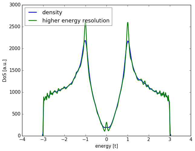
The accuracy in the energy resolution is dominated by the number of moments. The lowest accuracy is at the center of the spectrum, while slightly higher accuracy is obtained at the edges of the spectrum. If we use the KPM method (with the Jackson kernel, see Ref. [1]) to describe a delta peak at the center of the spectrum, we will obtain a function similar to a Gaussian of width \(σ=πa/N\), where \(N\) is the number of moments, and \(a\) is the width of the spectrum.
On the other hand, the random vectors will explore the range of the spectrum, and as the system gets bigger, the number of random vectors that are necessary to sample the whole spectrum reduces. Thus, a small number of random vectors is in general enough, and increasing this number will not result in a visible improvement of the approximation.
Our aim is to use the kernel polynomial method to obtain the spectral density \(ρ_A(E)\), as a function of the energy \(E\), of some Hilbert space operator \(A\). We define
where \(A(E)\) is the expectation value of \(A\) for all the eigenstates of the Hamiltonian with energy \(E\), and the density of states is
\(D\) being the Hilbert space dimension, and \(E_k\) the eigenvalues.
In the special case when \(A\) is the identity, then \(ρ_A(E)\) is simply \(ρ(E)\), the density of states.
In the following example, we will use the KPM implementation in Kwant to obtain the density of states of a graphene disk.
We start by importing kwant and defining our system.
# necessary imports
import kwant
import numpy as np


# define the system
def make_syst(r=30, t=-1, a=1):
    syst = kwant.Builder()
    lat = kwant.lattice.honeycomb(a, norbs=1)

    def circle(pos):
        x, y = pos
        return x ** 2 + y ** 2 < r ** 2

    syst[lat.shape(circle, (0, 0))] = 0.
    syst[lat.neighbors()] = t
    syst.eradicate_dangling()

    return syst
After making a system we can then create a SpectralDensity
object that represents the density of states for this system.
    fsyst = make_syst().finalized()

    spectrum = kwant.kpm.SpectralDensity(fsyst)
The SpectralDensity can then be called like a function to obtain a
sequence of energies in the spectrum of the Hamiltonian, and the corresponding
density of states at these energies.
energies, densities = spectrum()
When called with no arguments, an optimal set of energies is chosen (these are not evenly distributed over the spectrum, see Ref. [1] for details), however it is also possible to provide an explicit sequence of energies at which to evaluate the density of states.
    energy_subset = np.linspace(0, 2)
    density_subset = spectrum(energy_subset)

In addition to being called like functions, SpectralDensity
objects also have a method integrate which can be
used to integrate the density of states against some distribution function over
the whole spectrum. If no distribution function is specified, then the uniform
distribution is used:
print('identity resolution:', spectrum.integrate())
identity resolution: 6493.0
We see that the integral of the density of states is normalized to the total number of available states in the system. If we wish to calculate, say, the number of states populated in equilibrium, then we should integrate with respect to a Fermi-Dirac distribution:
    # Fermi energy 0.1 and temperature 0.2
    fermi = lambda E: 1 / (np.exp((E - 0.1) / 0.2) + 1)

    print('number of filled states:', spectrum.integrate(fermi))
number of filled states: 3274.13395902
The KPM method internally rescales the spectrum of the Hamiltonian to the
interval (-1, 1) (see Ref [1] for details), which requires calculating
the boundaries of the spectrum (using scipy.sparse.linalg.eigsh). This
can be very costly for large systems, so it is possible to pass this
explicitly as via the bounds parameter when instantiating the
SpectralDensity (see the class documentation for details).
Additionally, SpectralDensity accepts a parameter epsilon,
which ensures that the rescaled Hamiltonian (used internally), always has a
spectrum strictly contained in the interval (-1, 1). If bounds are not
provided then the tolerance on the bounds calculated with
scipy.sparse.linalg.eigsh is set to epsilon/2.
SpectralDensity has two methods for increasing the accuracy
of the method, each of which offers different levels of control over what
exactly is changed.
The simplest way to obtain a more accurate solution is to use the
add_moments method:
spectrum.add_moments(energy_resolution=0.03)
This will update the number of calculated moments and also the default
number of sampling points such that the maximum distance between successive
energy points is energy_resolution (see notes on accuracy).
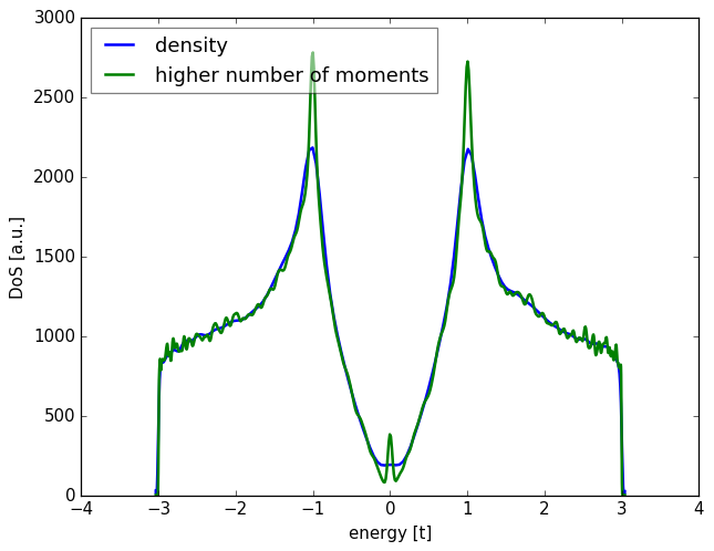
Alternatively, you can directly increase the number of moments
with add_moments, or the number of random vectors with add_vectors.
    spectrum.add_moments(100)
    spectrum.add_vectors(5)
Above, we saw how to calculate the density of states by creating a
SpectralDensity and passing it a finalized Kwant system.
When instantiating a SpectralDensity we may optionally
supply an operator in addition to the system. In this case it is
the spectral density of the given operator that is calculated.
SpectralDensity accepts the operators in a few formats:
kwant.operatorIf an explicit matrix is provided then it must have the same shape as the system Hamiltonian.
    # identity matrix
    matrix_op = scipy.sparse.eye(len(fsyst.sites))
    matrix_spectrum = kwant.kpm.SpectralDensity(fsyst, operator=matrix_op)
Or, to do the same calculation using kwant.operator.Density:
    # 'sum=True' means we sum over all the sites
    kwant_op = kwant.operator.Density(fsyst, sum=True)
    operator_spectrum = kwant.kpm.SpectralDensity(fsyst, operator=kwant_op)
Using operators from kwant.operator allows us to calculate quantities
such as the local density of states by telling the operator not to
sum over all the sites of the system:
    # 'sum=False' is the default, but we include it explicitly here for clarity.
    kwant_op = kwant.operator.Density(fsyst, sum=False)
    local_dos = kwant.kpm.SpectralDensity(fsyst, operator=kwant_op)
SpectralDensity will properly handle this vector output,
which allows us to plot the local density of states at different
point in the spectrum:
    zero_energy_ldos = local_dos(energy=0)
    finite_energy_ldos = local_dos(energy=1)

    _, axes = plt.subplots(1, 2, figsize=(12, 7))
    plot_ldos(fsyst, axes,[
        ('energy = 0', zero_energy_ldos),
        ('energy = 1', finite_energy_ldos),
    ])
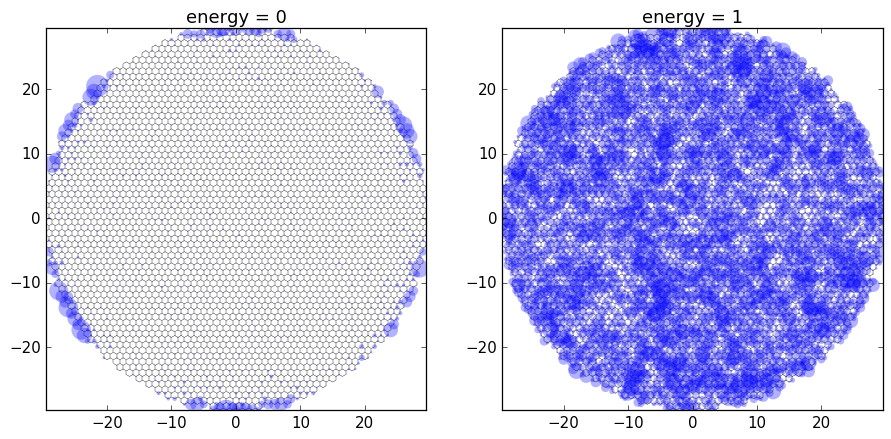
This nicely illustrates the edge states of the graphene dot at zero energy, and the bulk states at higher energy.
By default SpectralDensity will use random vectors
whose components are unit complex numbers with phases drawn
from a uniform distribution. There are several reasons why you may
wish to make a different choice of distribution for your random vectors,
for example to enforce certain symmetries or to only use real-valued vectors.
To change how the random vectors are generated, you need only specify a function that takes the dimension of the Hilbert space as a single parameter, and which returns a vector in that Hilbert space:
    # construct vectors with n random elements -1 or +1.
    def binary_vectors(n):
        return np.rint(np.random.random_sample(n)) * 2 - 1

    custom_factory = kwant.kpm.SpectralDensity(fsyst,
                                               vector_factory=binary_vectors)
Because KPM internally uses random vectors, running the same calculation
twice will not give bit-for-bit the same result. However, similarly to
the funcions in rmt, the random number generator can be directly
manipulated by passing a value to the rng parameter of
SpectralDensity. rng can itself be a random number generator,
or it may simply be a seed to pass to the numpy random number generator
(that is used internally by default).
Above, we showed how SpectralDensity can calculate the
spectral density of operators, and how we can define operators by using
kwant.operator. If you need even more flexibility,
SpectralDensity will also accept a function as its operator
parameter. This function must itself take two parameters, (bra, ket) and
must return either a scalar or a one-dimensional array. In order to be
meaningful the function must be a sesquilinear map, i.e. antilinear in its
first argument, and linear in its second argument. Below, we compare two
methods for computing the local density of states, one using
kwant.operator.Density, and the other using a custom function.
    rho = kwant.operator.Density(fsyst, sum=True)

    # sesquilinear map that does the same thing as `rho`
    def rho_alt(bra, ket):
        return np.vdot(bra, ket)

    rho_spectrum = kwant.kpm.SpectralDensity(fsyst, operator=rho)
    rho_alt_spectrum = kwant.kpm.SpectralDensity(fsyst, operator=rho_alt)
References
| [1] | (1, 2, 3, 4) Rev. Mod. Phys., Vol. 78, No. 1 (2006). |