Each of the following three examples highlights different ways to go beyond the very simple examples of the previous section.
See also
The complete source code of this example can be found in
tutorial/spin_orbit.py
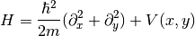
We begin by extending the simple 2DEG-Hamiltonian by a Rashba spin-orbit coupling and a Zeeman splitting due to an external magnetic field:

Here  denote the Pauli matrices.
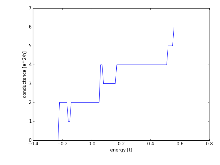
It turns out that this well studied Rashba-Hamiltonian has some peculiar properties in (ballistic) nanowires: It was first predicted theoretically in Phys. Rev. Lett. 90, 256601 (2003) that such a system should exhibit non-monotonic conductance steps due to a spin-orbit gap. Only very recently, this non-monotonic behavior has been supposedly observed in experiment: Nature Physics 6, 336 (2010). Here we will show that a very simple extension of our previous examples will exactly show this behavior (Note though that no care was taken to choose realistic parameters).
The tight-binding model corresponding to the Rashba-Hamiltonian naturally exhibits a 2x2-matrix structure of onsite energies and hoppings. In order to use matrices in our program, we import the Tinyarray package. (NumPy would work as well, but Tinyarray is much faster for small arrays.)
import tinyarray
For convenience, we define the Pauli-matrices first (with  the
unit matrix):
the
unit matrix):
sigma_0 = tinyarray.array([[1, 0], [0, 1]])
sigma_x = tinyarray.array([[0, 1], [1, 0]])
sigma_y = tinyarray.array([[0, -1j], [1j, 0]])
sigma_z = tinyarray.array([[1, 0], [0, -1]])
Previously, we used numbers as the values of our matrix elements.
However, Builder also accepts matrices as values, and
we can simply write:
    sys[(lat(x, y) for x in range(L) for y in range(W))] = \
        4 * t * sigma_0 + e_z * sigma_z
    # hoppings in x-direction
    sys[kwant.builder.HoppingKind((1, 0), lat, lat)] = \
        -t * sigma_0 - 1j * alpha * sigma_y
    # hoppings in y-directions
    sys[kwant.builder.HoppingKind((0, 1), lat, lat)] = \
        -t * sigma_0 + 1j * alpha * sigma_x
Note that the Zeeman energy adds to the onsite term, whereas the Rashba
spin-orbit term adds to the hoppings (due to the derivative operator).
Furthermore, the hoppings in x and y-direction have a different matrix
structure. We now cannot use lat.neighbors() to add all the hoppings at
once, since we now have to distinguish x and y-direction. Because of that, we
have to explicitly specify the hoppings in the form expected by
HoppingKind:
Since we are only dealing with a single lattice here, source and target lattice are identical, but still must be specified (for an example with hopping between different (sub)lattices, see Beyond square lattices: graphene).
Again, it is enough to specify one direction of the hopping (i.e.
when specifying (1, 0) it is not necessary to specify (-1, 0)),
Builder assures hermiticity.
The leads also allow for a matrix structure,
    lead[(lat(0, j) for j in xrange(W))] = 4 * t * sigma_0 + e_z * sigma_z
    # hoppings in x-direction
    lead[kwant.builder.HoppingKind((1, 0), lat, lat)] = \
        -t * sigma_0 - 1j * alpha * sigma_y
    # hoppings in y-directions
    lead[kwant.builder.HoppingKind((0, 1), lat, lat)] = \
        -t * sigma_0 + 1j * alpha * sigma_x
The remainder of the code is unchanged, and as a result we should obtain the following, clearly non-monotonic conductance steps:
The Tinyarray package, one of the dependencies of Kwant, implements efficient small arrays. It is used internally in Kwant for storing small vectors and matrices. For performance, it is preferable to define small arrays that are going to be used with Kwant using Tinyarray. However, NumPy would work as well:
import numpy
sigma_0 = numpy.array([[1, 0], [0, 1]])
sigma_x = numpy.array([[0, 1], [1, 0]])
sigma_y = numpy.array([[0, -1j], [1j, 0]])
sigma_z = numpy.array([[1, 0], [0, -1]])
Tinyarray arrays behave for most purposes like NumPy arrays except that they are immutable: they cannot be changed once created. This is important for Kwant: it allows them to be used directly as dictionary keys.
It should be emphasized that the relative hopping used for
HoppingKind is given in terms of
lattice indices, i.e. relative to the Bravais lattice vectors.
For a square lattice, the Bravais lattice vectors are simply
(a,0) and (0,a), and hence the mapping from
lattice indices (i,j) to real space and back is trivial.
This becomes more involved in more complicated lattices, where
the real-space directions corresponding to, for example, (1,0)
and (0,1) need not be orthogonal any more
(see Beyond square lattices: graphene).
See also
The complete source code of this example can be found in
tutorial/quantum_well.py
Up to now, all examples had position-independent matrix-elements (and thus translational invariance along the wire, which was the origin of the conductance steps). Now, we consider the case of a position-dependent potential:
The position-dependent potential enters in the onsite energies. One possibility would be to again set the onsite matrix elements of each lattice point individually (as in Transport through a quantum wire). However, changing the potential then implies the need to build up the system again.
Instead, we use a python function to define the onsite energies. We define the potential profile of a quantum well as:
def make_system(a=1, t=1.0, W=10, L=30, L_well=10):
    # Start with an empty tight-binding system and a single square lattice.
    # `a` is the lattice constant (by default set to 1 for simplicity.
    lat = kwant.lattice.square(a)

    sys = kwant.Builder()

    #### Define the scattering region. ####
    # Potential profile
    def potential(site, pot):
        (x, y) = site.pos
        if (L - L_well) / 2 < x < (L + L_well) / 2:
            return pot
        else:
            return 0
This function takes two arguments: the first of type Site,
from which you can get the real-space coordinates using site.pos, and the
value of the potential as the second. Note that in potential we can access
variables of the surrounding function: L and L_well are taken from the
namespace of make_system.
Kwant now allows us to pass a function as a value to
Builder:
    def onsite(site, pot=0):
        return 4 * t + potential(site, pot)

    sys[(lat(x, y) for x in range(L) for y in range(W))] = onsite
    sys[lat.neighbors()] = -t
For each lattice point, the corresponding site is then passed as the
first argument to the function onsite. The values of any additional
parameters, which can be used to alter the Hamiltonian matrix elements
at a later stage, are specified later during the call to smatrix.
Note that we had to define onsite, as it is
not possible to mix values and functions as in sys[...] = 4 * t +
potential.
For the leads, we just use constant values as before. If we passed a function also for the leads (which is perfectly allowed), this function would need to be compatible with the translational symmetry of the lead – this should be kept in mind.
Finally, we compute the transmission probability:
    # Compute conductance
    data = []
    for welldepth in welldepths:
        smatrix = kwant.smatrix(sys, energy, args=[-welldepth])
        data.append(smatrix.transmission(1, 0))

    pyplot.figure()
    pyplot.plot(welldepths, data)
    pyplot.xlabel("well depth [t]")
    pyplot.ylabel("conductance [e^2/h]")
    pyplot.show()
kwant.smatrix allows us to specify a list, args, that will be passed as
additional arguments to the functions that provide the Hamiltonian matrix
elements. In this example we are able to solve the system for different depths
of the potential well by passing the potential value. We obtain the result:
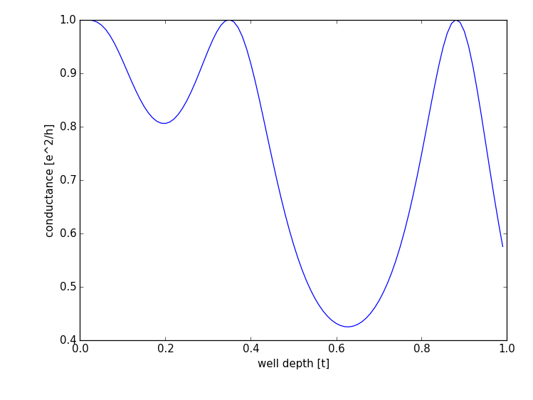
Starting from no potential (well depth = 0), we observe the typical oscillatory transmission behavior through resonances in the quantum well.
Warning
If functions are used to set values inside a lead, then they must satisfy the same symmetry as the lead does. There is (currently) no check and wrong results will be the consequence of a misbehaving function.
See also
The complete source code of this example can be found in
tutorial/ab_ring.py
Up to now, we only dealt with simple wire geometries. Now we turn to the case
of a more complex geometry, namely transport through a quantum ring
that is pierced by a magnetic flux  :
:

For a flux line, it is possible to choose a gauge such that a
charged particle acquires a phase  whenever it
crosses the branch cut originating from the flux line (branch
cut shown as red dashed line) [1]. There are more symmetric gauges, but
this one is most convenient to implement numerically.
whenever it
crosses the branch cut originating from the flux line (branch
cut shown as red dashed line) [1]. There are more symmetric gauges, but
this one is most convenient to implement numerically.
Defining such a complex structure adding individual lattice sites
is possible, but cumbersome. Fortunately, there is a more convenient solution:
First, define a boolean function defining the desired shape, i.e. a function
that returns True whenever a point is inside the shape, and
False otherwise:
def make_system(a=1, t=1.0, W=10, r1=10, r2=20):
    # Start with an empty tight-binding system and a single square lattice.
    # `a` is the lattice constant (by default set to 1 for simplicity).

    lat = kwant.lattice.square(a)

    sys = kwant.Builder()

    #### Define the scattering region. ####
    # Now, we aim for a more complex shape, namely a ring (or annulus)
    def ring(pos):
        (x, y) = pos
        rsq = x ** 2 + y ** 2
        return (r1 ** 2 < rsq < r2 ** 2)
Note that this function takes a real-space position as argument (not a
Site).
We can now simply add all of the lattice points inside this shape at once, using the function shape provided by the lattice:
    sys[lat.shape(ring, (0, r1 + 1))] = 4 * t
    sys[lat.neighbors()] = -t
Here, lat.shape takes as a second parameter a (real-space) point that is
inside the desired shape. The hoppings can still be added using
lat.neighbors() as before.
Up to now, the system contains constant hoppings and onsite energies,
and we still need to include the phase shift due to the magnetic flux.
This is done by overwriting the values of hoppings in x-direction
along the branch cut in the lower arm of the ring. For this we select
all hoppings in x-direction that are of the form (lat(1, j), lat(0, j))
with j<0:
    def fluxphase(site1, site2, phi):
        return exp(1j * phi)

    def crosses_branchcut(hop):
        ix0, iy0 = hop[0].tag

        # builder.HoppingKind with the argument (1, 0) below
        # returns hoppings ordered as ((i+1, j), (i, j))
        return iy0 < 0 and ix0 == 1  # ix1 == 0 then implied

    # Modify only those hopings in x-direction that cross the branch cut
    def hops_across_cut(sys):
        for hop in kwant.builder.HoppingKind((1, 0), lat, lat)(sys):
            if crosses_branchcut(hop):
                yield hop
    sys[hops_across_cut] = fluxphase
Here, crosses_branchcut is a boolean function that returns True for
the desired hoppings. We then use again a generator (this time with
an if-conditional) to set the value of all hoppings across
the branch cut to fluxphase. The rationale
behind using a function instead of a constant value for the hopping
is again that we want to vary the flux through the ring, without
constantly rebuilding the system – instead the flux is governed
by the parameter phi.
For the leads, we can also use the lat.shape-functionality:
    sym_lead = kwant.TranslationalSymmetry((-a, 0))
    lead = kwant.Builder(sym_lead)

    def lead_shape(pos):
        (x, y) = pos
        return (-W / 2 < y < W / 2)

    lead[lat.shape(lead_shape, (0, 0))] = 4 * t
    lead[lat.neighbors()] = -t
Here, the shape must be compatible with the translational symmetry
of the lead sym_lead. In particular, this means that it should extend to
infinity along the translational symmetry direction (note how there is
no restriction on x in lead_shape) [2].
Attaching the leads is done as before:
    sys.attach_lead(lead)
    sys.attach_lead(lead.reversed())
In fact, attaching leads seems not so simple any more for the current structure with a scattering region very much different from the lead shapes. However, the choice of unit cell together with the translational vector allows to place the lead unambiguously in real space – the unit cell is repeated infinitely many times in the direction and opposite to the direction of the translational vector. Kwant examines the lead starting from infinity and traces it back (going opposite to the direction of the translational vector) until it intersects the scattering region. At this intersection, the lead is attached:

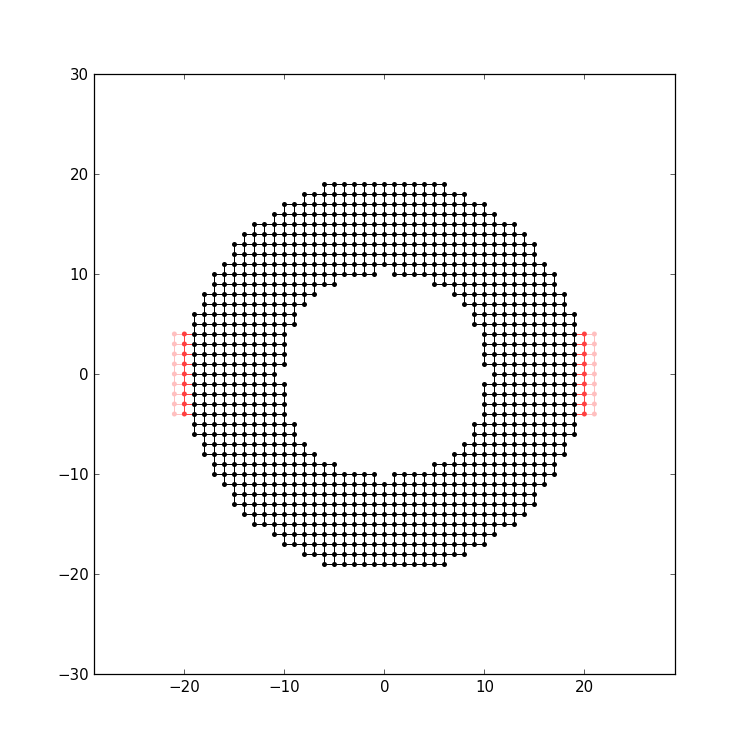
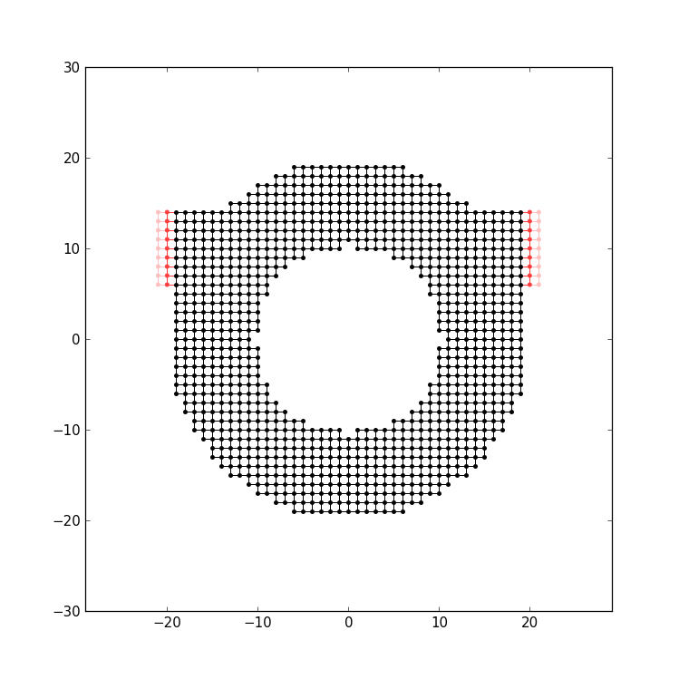
After the lead has been attached, the system should look like this:
The computation of the conductance goes in the same fashion as before. Finally you should get the following result:
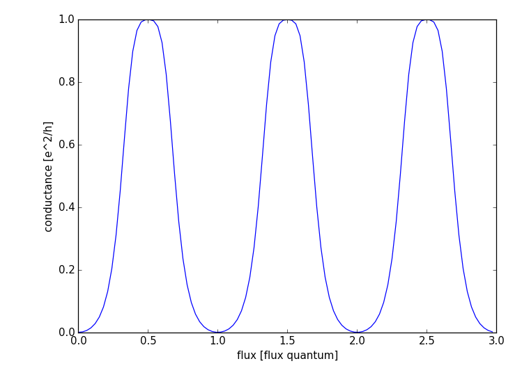
where one can observe the conductance oscillations with the period of one flux quantum.
Leads have to have proper periodicity. Furthermore, the Kwant
format requires the hopping from the leads to the scattering
region to be identical to the hoppings between unit cells in
the lead. attach_lead takes care of
all these details for you! In fact, it even adds points to
the scattering region, if proper attaching requires this. This
becomes more apparent if we attach the leads a bit further away
from the central axis o the ring, as was done in this example:
Per default, attach_lead attaches
the lead to the “outside” of the structure, by tracing the
lead backwards, coming from infinity.
One can also attach the lead to the inside of the structure, by providing an alternative starting point from where the lead is traced back:
sys.attach_lead(lead1, lat(0, 0))
starts the trace-back in the middle of the ring, resulting in the lead being attached to the inner circle:
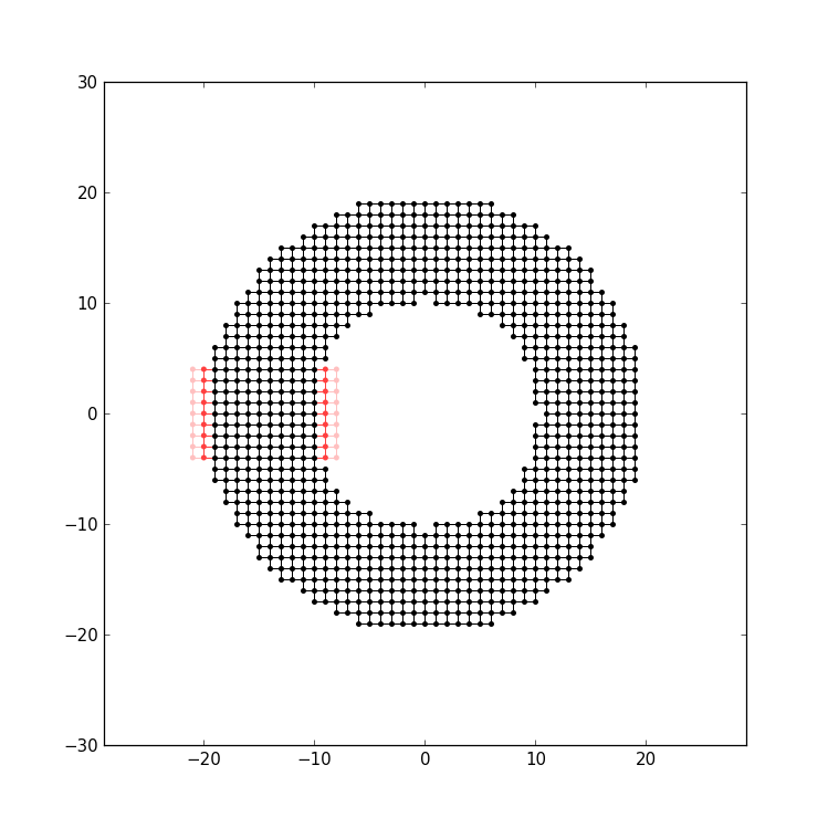
Note that here the lead is treated as if it would pass over the other arm of the ring, without intersecting it.
Footnotes
| [1] | The corresponding vector potential is  which yields the correct magnetic field which yields the correct magnetic field 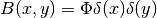 . . |
| [2] | Despite the “infinite” shape, the unit cell will still be finite; the
TranslationalSymmetry takes care of that. |