2.2. Getting started: a simple example with a one-dimensional chain
As a first simple example, we like to study the electron dynamics on an infinitly long one-dimensional chain consisting of nearest-neighbour coupled scatterers. Being initially at thermal equilibrium, we are intersted in the electron dynamics if a time-dependent perturbation \(V(t)\) acts on the one site with index zero. In second quantization the Hamiltonian is
The system looks like
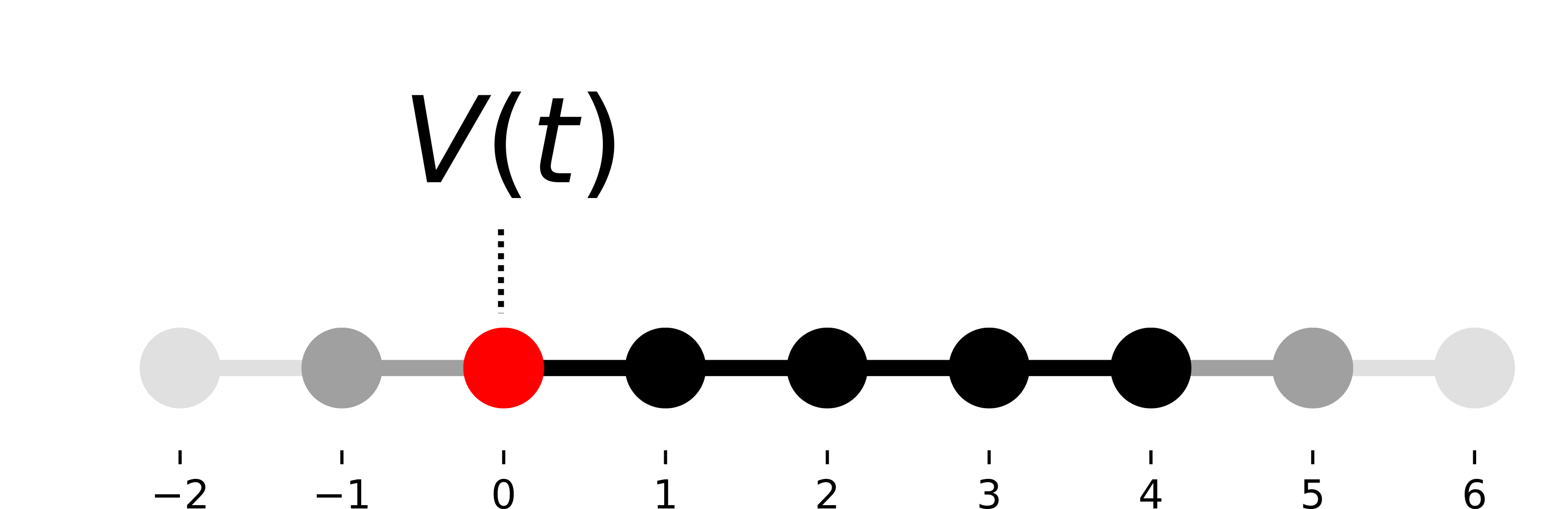
where the time-dependent onsite potential \(V(t)\) acts on the site with index zero (highlighted in red). The electron density will be calculated on the five central sites with indices 0 to 4. The sides with grey fading visualize the system extending to infinity on both sides. In this example, a simple linear function acts as the perturbation
Our observable is the onsite electron density
To use tkwant, the corresponding package must be loaded.
import tkwant
Also Kwant alongside with a few additional packages are required for the example.
import kwant
import numpy as np
import matplotlib.pyplot as plt
In the first step, the discretized tight-binding system is defined using Kwant. We expect that the reader is already familiar with Kwant and refer to the Kwant documentation for details. The one dimensional system with two semi-infinite leads attached on each site is defined by the following Kwant code
def make_system(length):

    def onsite_potential(site, time):
        return 1 + v(time)  # one is the static onsite element

    # system building
    lat = kwant.lattice.square(a=1, norbs=1)
    syst = kwant.Builder()

    # central scattering region
    syst[(lat(x, 0) for x in range(length))] = 1
    syst[lat.neighbors()] = -1
    # time dependent onsite-potential V(t) at leftmost site
    syst[lat(0, 0)] = onsite_potential

    # add leads
    sym = kwant.TranslationalSymmetry((-1, 0))
    lead_left = kwant.Builder(sym)
    lead_left[lat(0, 0)] = 1
    lead_left[lat.neighbors()] = -1
    syst.attach_lead(lead_left)
    syst.attach_lead(lead_left.reversed())

    return syst
We construct the system and finalize it, in order to allow numerical calculations.
syst = make_system(length=5).finalized()
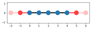
We can plot the system to have a first look. The length of 5 corresponds to the central scattering region (blue sites). The charge density will be evaluated on these sites and the time-dependent potential acts on the site with index zero. The two leads on the left and the right extend the chain to infinity (first sites are shown in red).
kwant.plot(syst);
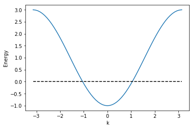
By default, tkwant treats the translationally invariant leads to be at thermal equilibrium with a temperature \(T = 0\), and a chemical potential \(\mu = 0\). The dispersion of the lead spectrum in the first Brillouine zone is plotted below (blue, straight) with the Fermi level (black, dashed). The occupied states are below the Fermi energy.
chemical_potential = 0
kwant.plotter.bands(syst.leads[0], show=False)
plt.plot([-np.pi, np.pi], [chemical_potential] * 2, 'k--')
plt.show()
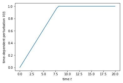
The time dependent perturbation \(V(t)\) is written as
def v(time, tau=8):
    if time < tau:
        return time / tau
    return 1
and its plot is
times = np.linspace(0, 20)
plt.plot(times, [v(t) for t in times])
plt.xlabel(r'time $t$')
plt.ylabel(r'time-dependent perturbation $V(t)$')
plt.show()
The density expectation value at the central sites is directly available by the corresponding Kwant operator
density_operator = kwant.operator.Density(syst)
To perform the actual tkwant simulation, we first initialize the
many-body state. The evolve() and evaluate() methods propagate
the state foreward in time and evaluate the manybody expectation value.
state = tkwant.manybody.State(syst, tmax=max(times))

densities = []
for time in times:
    state.evolve(time)
    density = state.evaluate(density_operator)
    densities.append(density)
This was already the entire simulation. We finally plot the result
densities = np.array(densities).T
for site, density in enumerate(densities):
    plt.plot(times, density, label='site {}'.format(site))
plt.xlabel(r'time $t$')
plt.ylabel(r'charge density $n$')
plt.legend()
plt.show()
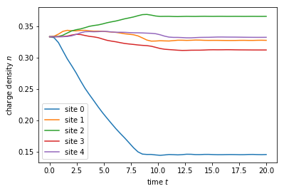
Starting from equilibrium at initial time \(t = 0\) where the density is equal on all sites, it evolves to different vales when the perturbation is switched on. After some transient regime, the density reaches stationary values at long times.
See also
The complete source code of this example can be found in
1d_wire_onsite.py