2. kwantSpectrum tutorial
For many situations we need to calculate and analyze the band structure of a semi-infinite lead. In the following we will look at a simple toy model with three crossing bands.
import numpy as np
import matplotlib.pyplot as plt
from functools import partial

import kwant
from kwant.physics import dispersion

def make_lead_with_crossing_bands():
    lat = kwant.lattice.square(1, norbs=1)
    sym = kwant.TranslationalSymmetry((-2, 0))
    H = kwant.Builder(sym)
    H[lat(0, 0)] = 0
    H[lat(0, 1)] = 0
    H[lat(1, 0)] = 0
    H[lat(1, 0), lat(0, 0)] = 1
    H[lat(2, 1), lat(0, 1)] = 1
    H[lat(2, 0), lat(1, 0)] = 0.5
    return H

lead = make_lead_with_crossing_bands().finalized()
2.1. Basic band structure calculation
The most direct way to obtain the spectrum of a lead is to diagonalize
its Hamiltonian matrix. This is implemented in the class Bands:
bands = dispersion.Bands(lead)
An instance of the Bands class can be called with a momentum value
to obtain the energies of all open modes. The different modes are
ordered according to their respective energy value. The first and second
derivative (velocity and curvature) can be calculated by specifying the
keyword derivative_order (derivative_order = 0 by default). With
derivative_order= 1 or 2 the first and respectively second order
derivative are returned in addition to the energy.
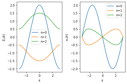
In the following example we plot the energies \(E_m(k)\) and velocities \(\partial_k E_m(k) = v_m(k)\) for our testcase, where \(k\) is the momentum and \(m\) is the mode index. Note that the band dispersion \(E_m(k)\) is discontinuously colored and the velocity \(v_m(k)\) has discontinous jumps, since the mode index \(m\) changes when two bands cross.
momenta = np.linspace(-np.pi, np.pi, 500)

plt.subplot(1, 2, 1)
energies = [bands(k) for k in momenta]
plt.plot(momenta, energies)
plt.xlabel(r'$k$')
plt.ylabel(r'$E_m(k)$')

plt.subplot(1, 2, 2)
velocities = [bands(k, derivative_order=1)[1] for k in momenta]
plt.plot(momenta, velocities)
plt.xlabel(r'$k$')
plt.ylabel(r'$v_m(k)$')

plt.tight_layout()
plt.show()
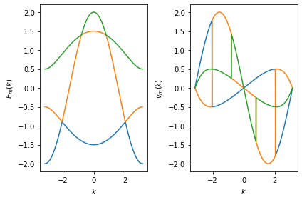
Without plotting the spectrum and and the manual ordering of the bands,
it is not possible to directly obtain continuous bands from Bands.
2.2. Analysis of the band structure
A much more convenient method for examining the spectrum is the
spectrum() function. It is used quite similar:
import kwantspectrum as ks

spec = ks.spectrum(lead)
The spectrum() function returns an object (spec in the
current example) and we will refer to this object in the following
simply as the instance of spectrum(). One can call the spec
instance with a momentum (\(k\)) to directly calculate the energy
dispersion \(\partial_k^d E_n(k)\) or its derivatives. The
derivative order (\(d\)) is set by the keyword derivative_order
(derivative_order = 0 by default) and the band index \(n\) can
be passed with the keyword band. If band is not specified, the
result is returned for all \(N\) bands. The total number of bands
(\(N\)) is also accessible via the instance attribute nbands.
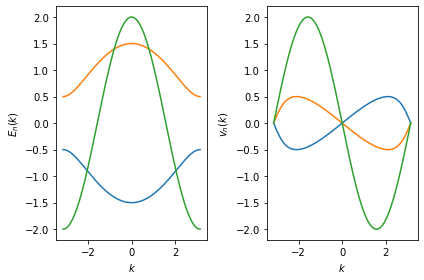
In the following example, we recalculate the energies \(E_n(k)\) and velocities \(\partial_k E_n(k) = v_n(k)\) for our test case:
plt.subplot(1, 2, 1)
for band in range(spec.nbands):
    plt.plot(momenta, spec(momenta, band), label='n=' + str(band))
plt.xlabel(r'$k$')
plt.ylabel(r'$E_n(k)$')
plt.legend()

plt.subplot(1, 2, 2)
for band in range(spec.nbands):
    plt.plot(momenta, spec(momenta, band, derivative_order=1), label='n=' + str(band))
plt.xlabel(r'$k$')
plt.ylabel(r'$v_n(k)$')
plt.legend()

plt.tight_layout()
plt.show()
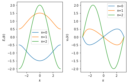
Note that the different bands are now represented as continous functions
\(E_n(k)\) uniquely identified by the discrete band index \(n\)
and the continuous momentum \(k\). By default, the bands are ordered
at the momentum \(k=0\). The band with the lowest energy has the
index \(n = 0\) and the index increases with increasing energy up to
\(n = N - 1\), where \(N\) is the total number of bands.
Moreover, the spec instance can be called directly with an array
of momentum (\(k\)) values.
2.2.1. Intervals and intersections
The spec instance provides two methods two analyze the spectrum:
intersect and intervals.
The intersect method returns all momentum (\(k\)) points that
solve the equation
The band index \(n\) is passed with the keyword band. The
derivative order (\(d\)) is set by the keyword derivative_order
(derivative_order = 0 by default). \(f(k)\) can be either a
callable function or a scalar numeric value. In the following example we
use intersect to find for each band the momentum points where: the
dispersion has an energy of \(\pm 1\) (green points), the dispersion
has local minima or maxima (blue points), and finally the dispersion has
an inflection point (red points).
plt.plot(momenta, spec(momenta), '--k', alpha=0.4)
lower, upper = -1, 1

for band in range(spec.nbands):
    cross = spec.intersect(lower, band)
    if cross.size > 0:
        plt.plot(cross, spec(cross, band), 'go')
    cross = spec.intersect(upper, band)
    if cross.size > 0:
        plt.plot(cross, spec(cross, band), 'go')

    velocity_zeros = spec.intersect(0, band, derivative_order=1)
    plt.plot(velocity_zeros, spec(velocity_zeros, band), 'bo')

    curvature_zeros = spec.intersect(0, band, derivative_order=2)
    plt.plot(curvature_zeros, spec(curvature_zeros, band), 'ro')

plt.plot([-np.pi, np.pi],[[lower, upper], [lower, upper]], '--k')
plt.xlabel(r'$k$')
plt.ylabel(r'$E_n(k)$')
plt.show()
The method intervals() returns a list of momentum (\(k\))
intervals that solves the equation
The derivative order (\(d\)) is set by the keyword
derivative_order (derivative_order = 0 by default) and the band
index \(n\) is passed by the keyword band. Upper and lower
bounds must be constant scalar values (set via upper and lower).
They can also be partially skipped to define only an upper or
respectively lower limit.
The function intersect_intervals() can be used to obtain a list of
all overlapping intervals from two lists of intervals.
In the following example we find the momentum intervals where the band energy is between the limits \([-1, 1]\) and also the velocity is positive.
plt.plot(momenta, spec(momenta), '--k', alpha=0.4)

for band in range(spec.nbands):
    intervals_e = spec.intervals(band, lower=lower, upper=upper)
    intervals_v = spec.intervals(band, lower=0, derivative_order=1)
    intervals = ks.intersect_intervals(intervals_e, intervals_v)
    for interval in intervals:
        k = np.linspace(*interval)
        plt.plot(k, spec(k, band), 'k', linewidth=3.0)

plt.plot([-np.pi, np.pi],[[lower, upper], [lower, upper]], '--k')
plt.xlabel(r'$k$')
plt.ylabel(r'$E_n(k)$')
plt.show()

2.2.2. Order point
By defaut, the bands are ordered at momentum \(k = 0\), whereby the
band with the lowest energy has the index 0. We can change the reference
momentum where the bands are ordered with the keyword orderpoint.
In the following example, we order the bands at momentum \(k = -\pi\):
spec = ks.spectrum(lead, orderpoint=-np.pi)

plt.subplot(1, 2, 1)
for band in range(spec.nbands):
    plt.plot(momenta, spec(momenta, band), label='n=' + str(band))
plt.xlabel(r'$k$')
plt.ylabel(r'$E_n(k)$')
plt.legend()

plt.subplot(1, 2, 2)
for band in range(spec.nbands):
    plt.plot(momenta, spec(momenta, band, derivative_order=1), label='n=' + str(band))
plt.xlabel(r'$k$')
plt.ylabel(r'$v_n(k)$')
plt.legend()

plt.tight_layout()
plt.show()
2.2.3. Sampling region and periodicity
spectrum() assumes a periodic spectrum, \(E_n(k) = E_n(k + K)\)
with a (default) period length \(K = 2 \pi\). To archive this,
spectrum() analyzes the spectrum \(E_n(k)\) in the first
Brillouin zone in a \([- \pi, \pi]\) interval. If the instance of
spectrum() is then called with a momentum
\(k \not\in [- \pi, \pi]\), the momentum argument \(k\) is
periodically mapped into the \([- \pi, \pi]\) interval, in which
\(E_n(k)\) was first analyzed. This assignment is possible if the
first sampling range is same or greater than the period length
\(K\). By default, this is the case and a spec instance can
therefore be called with any momentum value
\(k \in [- \infty, \infty]\).
The two methods intersections() and intervals() return their
values by default in range of the analyzation interval, which is
\([- \pi, \pi]\) by default. One can change this behavior to get
intervals and crossings within a given \([k_{min}, k_{max}]\) range
by specifying kmin and kmax when calling the intersect() or
the intervals() method. As before, kmin and kmax can take
any value from \(- \infty\) to \(\infty\) as long as initial
sampling range is equal or greater than the period.
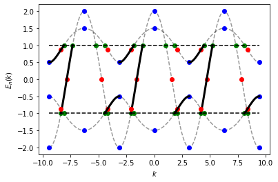
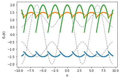
In the following example, we analyse the spectrum on an enlarged \([-3 \pi, 3 \pi]\) interval. The initial sampling interval (on \([- \pi, \pi]\) ) and the periodicity (\(K = 2 \pi\)) are both default values. As before, crossings with the upper and the lower limit (green), velocity zeros (blue) and inflection points (red) are highlighted. We also extract the intervals with a positive velocity between the upper and the lower limit (black solid line).
lower, upper = -1, 1
kmin, kmax = - 3 * np.pi, 3* np.pi

momenta = np.linspace(kmin, kmax, 500)
plt.plot(momenta, spec(momenta), '--k', alpha=0.4)

for band in range(spec.nbands):
    cross = spec.intersect(lower, band, kmin=kmin, kmax=kmax)
    if cross.size > 0:
        plt.plot(cross, spec(cross, band), 'go')
    cross = spec.intersect(upper, band, kmin=kmin, kmax=kmax)
    if cross.size > 0:
        plt.plot(cross, spec(cross, band), 'go')

    velocity_zeros = spec.intersect(0, band, derivative_order=1, kmin=kmin, kmax=kmax)
    plt.plot(velocity_zeros, spec(velocity_zeros, band), 'bo')

    curvature_zeros = spec.intersect(0, band, derivative_order=2, kmin=kmin, kmax=kmax)
    plt.plot(curvature_zeros, spec(curvature_zeros, band), 'ro')

    ie = spec.intervals(band, lower=lower, upper=upper, kmin=kmin, kmax=kmax)
    iv = spec.intervals(band, lower=0, derivative_order=1, kmin=kmin, kmax=kmax)
    intervals = ks.intersect_intervals(ie, iv)
    for interval in intervals:
        k = np.linspace(*interval)
        plt.plot(k, spec(k, band), 'k', linewidth=3.0)

plt.plot([kmin, kmax],[lower, lower], '--k')
plt.plot([kmin, kmax],[upper, upper], '--k')
plt.xlabel(r'$k$')
plt.ylabel(r'$E_n(k)$')
plt.show()
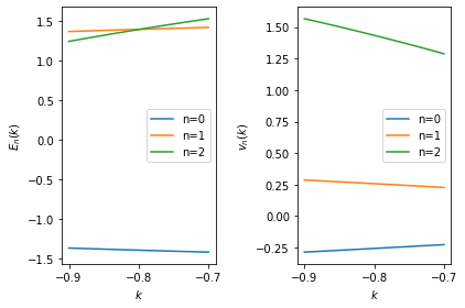
One can change the initial analysis interval \([k_{min}, k_{max}]\)
used when calling spectrum() by passing kmin and kmax. By
default, the initial sampling interval is \([-\pi, \pi]\). Changing
the intitial sampling interval can be interesting if, for example, one
likes to concentrate on a particular region of a spectrum in a
complicated system.
In the following example, we analyze the spectrum within the \([-0.9, -0.7]\) interval around an intersection:
kmin, kmax = -0.9, -0.7
spec = ks.spectrum(lead, kmin=kmin, kmax=kmax)
momenta = np.linspace(kmin, kmax)

plt.subplot(1, 2, 1)
for band in range(spec.nbands):
    plt.plot(momenta, spec(momenta, band), label='n=' + str(band))
plt.xlabel(r'$k$')
plt.ylabel(r'$E_n(k)$')
plt.legend()

plt.subplot(1, 2, 2)
for band in range(spec.nbands):
    plt.plot(momenta, spec(momenta, band, derivative_order=1), label='n=' + str(band))
plt.xlabel(r'$k$')
plt.ylabel(r'$v_n(k)$')
plt.legend()

plt.tight_layout()
plt.show()
plt.show()
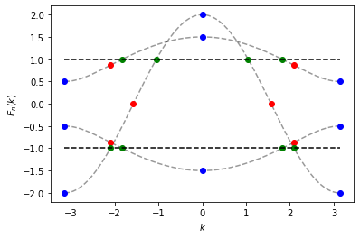
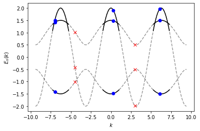
Our spectrum is considered perodic, \(E_n(k) = E_n(k + K)\), with period length \(K\) and \(E_n(k)\) has been analyzed for \(k \in [k_{min}, k_{max}]\). If the length of the sampling interval is less than the period length, \(k_{max} - k_{min} < K\), we can only map \(k\) to the analyzed values if
where \(j\) labels the periodic images.
To show this in an example, we create an spec instance named
spec_short in the following, that samples \(E_n(k)\) on a
\([-1, 1]\) interval. Since the sampling region is smaller than the
(default) period length \(K = 2 \pi\), we can only evaluate
spec_short for momenta \(k \in [-1, 1]\) and the respective
mirror regions \(k \in [-1\pm 2 j \pi, 1\pm 2 j \pi]\) (represented
by the black lines for \(j = 1\)). The three momentum points
(represented by blue points), are valid arguments for
spec_short, because they fall into one of these three intervals.
However, it is not possible to evaluate spec_short at points
outsite these intervals (e.g. the two random points marked by red
crosses). As a guide for the eye, the entire spectrum over three periods
is represented by dashed grey lines.
# reference spectrum (sample interval = period length)
spec = ks.spectrum(lead)
momenta = np.linspace(-3*np.pi, 3*np.pi, 500)
random_points_outside = [-4.5, 3]
plt.plot(momenta, spec(momenta), '--k', alpha=0.4)
plt.plot(random_points_outside, spec(random_points_outside), 'xr')

# sample the spectrum on smaller intervall (sample interval < period length)
kmin, kmax = -1, 1
momenta = np.linspace(kmin, kmax)
spec_short = ks.spectrum(lead, kmin=kmin, kmax=kmax)
period_len = 2 * np.pi
random_points_inside = [-7, 0.3, 6.1]
plt.plot(momenta, spec_short(momenta), 'k')
plt.plot(momenta - period_len, spec_short(momenta - period_len), 'k')
plt.plot(momenta + period_len, spec_short(momenta + period_len), 'k')
plt.plot(random_points_inside, spec_short(random_points_inside), 'ob')
plt.xlabel(r'$k$')
plt.ylabel(r'$E_n(k)$')
plt.show()
If the Brillouin zone of our system has a different periodicity
\(K\) than the default \(2 \pi\) setting, we can transfer the
periodicity information with the keyword period. In this case
period=\((l, u)\) is a tuple where \(l\) is the lower
and \(u\) the limit of a periodic range. The periodic length is
defined as \(K = u - l\). If period = False, no perodic
assignment is applied to \(k\) at all.
In the following example, we show how to change the periodicity of the
ks. The spectrum is initially analyzed in the (default)
\([- \pi, \pi]\) interval when the spec instance is created.
We then evaluate the spectrum for two different periodicities, when
calling this instance. First we evaluate the spectrum with the default
\(K = 2 \pi\) periodic length (grey dashed). Second, we evaluate the
spectrum as a function that is assumed to be periodic on a
\([-1.5, 1]\) interval (blue, orange and green solid line), so that
the periodic length is \(K = 2.5\). The initial analyzation interval
is equal (in the first case) or greater (in the second case) than
\(K\), so we can plot the spectrum for all
\(k \in [- \infty, \infty]\).
momenta = np.linspace(-3*np.pi, 3*np.pi, 5000)
plt.plot(momenta, spec(momenta), '--k', alpha=0.4)  # periodic on [-pi, pi]
spec.set_period((-1.5, 1))
for band in range(spec.nbands):
    plt.plot(momenta, spec(momenta, band), 'o', markersize=1)  # periodic on [-1.5, 1]
plt.xlabel(r'$k$')
plt.ylabel(r'$E_n(k)$')
plt.show()
For representation purpose, we plot discrete points in this example to avoid adding interfering connecting lines during discontious jumps.
2.2.4. Retrieve evaluation points and ordering vectors
When calling spectrum(), the different bands are first ordered on a
set of discrete momentum points selected by an adaptive algorithm. In a
second step, the discrete points are interpolated (currently by
piecewise cubic Hermite splines). Subsequent calls of a spec
instance only evaluate the interpolation function. However, we can
retrieve the original points selected by the ordering algorithm.
Momentum \((k)\) points, energies \(E_n(k)\) and velocities
\(v_n(k)\) are stored in the instance attributes x, y and
dy.
In the following example, we plot the energies \(E_n(k)\) and velocities \(v_n(k)\) selected by the adaptive ordering algorithm:
plt.subplot(1, 2, 1)
plt.plot(spec.x, spec.y)
plt.xlabel(r'$k$')
plt.ylabel(r'$E_n(k)$')


plt.subplot(1, 2, 2)
plt.plot(spec.x, spec.dy)
plt.xlabel(r'$k$')
plt.ylabel(r'$v_n(k)$')

plt.tight_layout()
plt.show()
We can also get the ordering vector that stores the information on how
spectrum() reordered the output of Bands on the internally
stored \(k\) points.
In the following example, we reorder the energies and velocities of
Bands to get the order similar to spectrum():
energies = [bands(k)[order] for k, order in zip(spec.x, spec.ordering)]

plt.subplot(1, 2, 1)
plt.plot(spec.x, energies)
plt.xlabel(r'$k$')
plt.ylabel(r'$E_n(k)$')

velocities = [bands(k, derivative_order=1)[1][order] for k, order
              in zip(spec.x, spec.ordering)]

plt.subplot(1, 2, 2)
plt.plot(spec.x, velocities)
plt.xlabel(r'$k$')
plt.ylabel(r'$v_n(k)$')

plt.tight_layout()
plt.show()

2.2.5. Accuracy
We can adjust the numerical accuracy (with keyword tol) to change
the number evaluation points used internally.
for tol in [1E-4, 1E-8]:
    spec = ks.spectrum(lead, tol=tol)
    print('tolerance= {}, number of points= {}'.format(tol, len(spec.x)))
tolerance= 0.0001, number of points= 57
tolerance= 1e-08, number of points= 577
Note that tol affects both the matching and the interpolation step.
First, if the tolerance becomes too large, the internally used matching
algorithm (see _match_functions below) may no longer be able to
match the corresponding bands correctly. Second, the interpolation,
which is used when an spec instance or instance methods are
called changes its accuracy when the number of evaluation points
changes. As mentioned earlier, one can always retrieve the internally
stored values (x, y and dy), where \(E_n(k)\) and
\(v_n(k)\) correspond to the exact diagonalization result.
2.3. Matching algorithm
To understand how spectrum() work, we will play directly with the
underlying matching algorithm implemented in _match_functions. We
will only show the usage here, but refer to the technical documentation
for further explanation. (TODO: insert link)
2.3.1. Avoided-crossing model
We will apply the matching algorithm to a simplified model function that physically mimics the avoided crossing of two bands.
At \(x = x_0\) the two functions have a distance (finite gap) of size \(2 \Delta\). While in the analytical form it is trivial to distinguish between the two functions \(f_1\) and \(f_2\), it is a nontrivial problem to directly match the function values together, which on a given point \(x\) belong either to \(f_1\) and \(f_2\). We assume in the following that our function are continous and sufficiently smooth, when evaluated on a finite set of discrete points.
def gap_function(x, gap, x0):
    dx = x - x0
    xsqrt = np.sqrt(dx * dx + gap * gap)

    def f(x):
        return xsqrt

    def df(x):
        return dx / xsqrt

    return np.array([[f(x), -f(x)], [df(x), -df(x)]])
The function gap_function calculates \(f_1\) and \(f_2\) as
well as the first derivatives. Again, while it is trivial to see that
\(f_1\) and \(f_2\) belong always to the first and the second
element of the return vector of gap_function, we cannot see this if
we only look at the evaluated function values of gap_function. We
now use the matching algorithm for different sizes of the gap value.
While we look at a symmetric interval [-1, 1] to perform the matching,
we set the gap “off” the center closer to the right edge. Otherwise, if
the gap is kept exactly in the middle of the interval, the algorithm
always finds the gap in a first nesting step.
tol = 1e-3

for i, gap in enumerate([1E-1, 1E-2, 1E-3]):
    func = partial(gap_function, gap=gap, x0=0.3)
    x, y, dy, *_ = ks._match_functions(func, xmin=-1, xmax=1, tol=tol, min_iter=1)

    plt.subplot(1, 3, i+1)
    plt.plot(x, y, '--o')
    plt.title("gap = {}".format(gap))
plt.tight_layout()
plt.show()
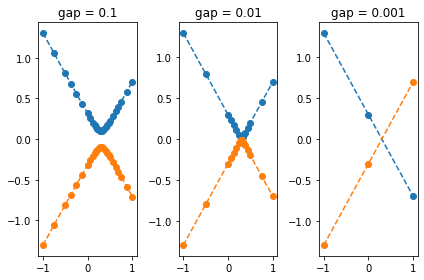
The above example shows that the gap is correctly identified in the
first two cases, while in the last case it is overlooked for the
smallest gap value. We can increase the tolerance with the keyword
tol such that the gap is as well identified in the last case:
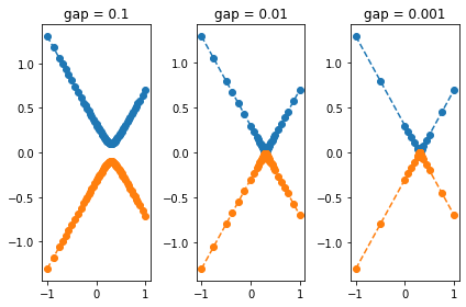
tol = 1e-5

for i, gap in enumerate([1E-1, 1E-2, 1E-3]):
    func = partial(gap_function, gap=gap, x0=0.3)
    x, y, dy, *_ = ks._match_functions(func, xmin=-1, xmax=1, tol=tol, min_iter=1)

    plt.subplot(1, 3, i+1)
    plt.plot(x, y, '--o')
    plt.title("gap = {}".format(gap))
plt.tight_layout()
plt.show()
While the algorithm can always fail with more complicated examples and assign functions wrongly, is more likely to overlook an avoided crossing, then to actually miss an intersection, as shown here.
2.3.2. Random order
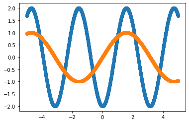
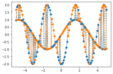
In the next example we consider a vector function \(f(x) = (\sin(x), -2 \cos(x))^T\) where we randomly reverse the order of the two vector components at each function call.
def model_func(xx):
    def f(x):
        return np.array([np.sin(x), -2*np.cos(2*x)])

    def df(x):
        return np.array([np.cos(x), 4*np.sin(2*x)])

    ran = np.random.randint(2, size=1)[0]
    order = np.array([ran, 1 - ran])

    return np.array([f(xx)[order], df(xx)[order]])
A plot of the function could look like this
xx = np.linspace(-5, 5, 100)
yy = [model_func(x)[0] for x in xx]
plt.plot(xx, yy, '--o')
plt.show()
Using the matching algorithm, we can reconstruct the order with respect to the original continous vector function
xx, yy, dyy, *_ = ks._match_functions(model_func, xmin=-5, xmax=5, min_iter=1)
plt.plot(xx, yy, '--o')
plt.show()