In the previous tutorials we have mainly concentrated on calculating global
properties such as conductance and band structures. Often, however, insight can
be gained from calculating locally-defined quantities, that is, quantities
defined over individual sites or hoppings in your system. In the
Closed systems tutorial we saw how we could visualize the density
associated with the eigenstates of a system using kwant.plotter.map.
In this tutorial we will see how we can calculate more general quantities than simple densities by studying spin transport in a system with a magnetic texture.
See also
The complete source code of this example can be found in
magnetic_texture.py
Our starting point will be the following spinful tight-binding model on a square lattice:
where latin indices run over sites, and greek indices run over spin. We can identify the first term as a nearest-neighbor hopping between like-spins, and the second as a term that couples spins on the same site. The second term acts like a magnetic field of strength \(J\) that varies from site to site and that, on site \(i\), points in the direction of the unit vector \(\mathbf{m}_i\). \(\mathbf{σ}_{αβ}\) is a vector of Pauli matrices. We shall take the following form for \(\mathbf{m}_i\):
where \(x_i\) and \(y_i\) are the \(x\) and \(y\) coordinates of site \(i\), and \(r_i = \sqrt{x_i^2 + y_i^2}\).
To define this model in Kwant we start as usual by defining functions that depend on the model parameters:
def field_direction(pos, r0, delta):
    x, y = pos
    r = np.linalg.norm(pos)
    r_tilde = (r - r0) / delta
    theta = (tanh(r_tilde) - 1) * (pi / 2)

    if r == 0:
        m_i = [0, 0, -1]
    else:
        m_i = [
            (x / r) * sin(theta),
            (y / r) * sin(theta),
            cos(theta),
        ]

    return np.array(m_i)


def scattering_onsite(site, r0, delta, J):
    m_i = field_direction(site.pos, r0, delta)
    return J * np.dot(m_i, sigma)


def lead_onsite(site, J):
    return J * sigma_z
and define our system as a square shape on a square lattice with two orbitals per site, with leads attached on the left and right:
lat = kwant.lattice.square(norbs=2)

def make_system(L=80):

    syst = kwant.Builder()

    def square(pos):
        return all(-L/2 < p < L/2 for p in pos)

    syst[lat.shape(square, (0, 0))] = scattering_onsite
    syst[lat.neighbors()] = -sigma_0

    lead = kwant.Builder(kwant.TranslationalSymmetry((-1, 0)),
                         conservation_law=-sigma_z)

    lead[lat.shape(square, (0, 0))] = lead_onsite
    lead[lat.neighbors()] = -sigma_0

    syst.attach_lead(lead)
    syst.attach_lead(lead.reversed())

    return syst
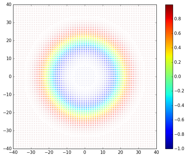
Below is a plot of a projection of \(\mathbf{m}_i\) onto the x-y plane inside the scattering region. The z component is shown by the color scale:
We will now be interested in analyzing the form of the scattering states that originate from the left lead:
    params = dict(r0=20, delta=10, J=1)
    wf = kwant.wave_function(syst, energy=-1, params=params)
    psi = wf(0)[0]
If we were simulating a spinless system with only a single degree of freedom, then calculating the density on each site would be as simple as calculating the absolute square of the wavefunction like:
density = np.abs(psi)**2
When there are multiple degrees of freedom per site, however, one has to be more careful. In the present case with two (spin) degrees of freedom per site one could calculate the per-site density like:
    # even (odd) indices correspond to spin up (down)
    up, down = psi[::2], psi[1::2]
    density = np.abs(up)**2 + np.abs(down)**2
With more than one degree of freedom per site we have more freedom as to what local quantities we can meaningfully compute. For example, we may wish to calculate the local z-projected spin density. We could calculate this in the following way:
    # spin down components have a minus sign
    spin_z = np.abs(up)**2 - np.abs(down)**2
If we wanted instead to calculate the local y-projected spin density, we would need to use an even more complicated expression:
    # spin down components have a minus sign
    spin_y = 1j * (down.conjugate() * up - up.conjugate() * down)
The kwant.operator module aims to alleviate somewhat this tedious
book-keeping by providing a simple interface for defining operators that act on
wavefunctions. To calculate the above quantities we would use the
Density operator like so:
    rho = kwant.operator.Density(syst)
    rho_sz = kwant.operator.Density(syst, sigma_z)
    rho_sy = kwant.operator.Density(syst, sigma_y)

    # calculate the expectation values of the operators with 'psi'
    density = rho(psi)
    spin_z = rho_sz(psi)
    spin_y = rho_sy(psi)
Density takes a System as its first parameter
as well as (optionally) a square matrix that defines the quantity that you wish
to calculate per site. When an instance of a Density is then
evaluated with a wavefunction, the quantity
is calculated for each site \(i\), where \(\mathbf{ψ}_{i}\) is a vector consisting of the wavefunction components on that site and \(\mathbf{M}\) is the square matrix referred to previously.
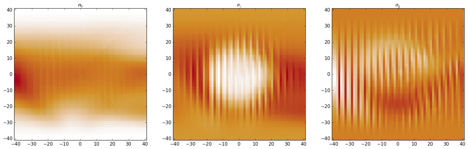
Below we can see colorplots of the above-calculated quantities. The array that
is returned by evaluating a Density can be used directly with
kwant.plotter.map:
Although we refer loosely to “densities” and “operators” above, a
Density actually represents a collection of linear
operators. This can be made clear by rewriting the above definition
of \(ρ_i\) in the following way:
where greek indices run over the degrees of freedom in the Hilbert space of the scattering region and latin indices run over sites. We can this identify \(\mathcal{M}_{iαβ}\) as the components of a rank-3 tensor and can represent them as a “vector of matrices”:
where \(\mathbf{M}\) is defined as in the main text, and the \(0\) are zero matrices of the same shape as \(\mathbf{M}\).
kwant.operator also has a class Current for calculating
local currents, analogously to the local “densities” described above. If
one has defined a density via a matrix \(\mathbf{M}\) and the above
equation, then one can define a local current flowing from site \(b\)
to site \(a\):
where \(\mathbf{H}_{ab}\) is the hopping matrix from site \(b\) to site \(a\). For example, to calculate the local current and spin current:
    J_0 = kwant.operator.Current(syst)
    J_z = kwant.operator.Current(syst, sigma_z)
    J_y = kwant.operator.Current(syst, sigma_y)

    # calculate the expectation values of the operators with 'psi'
    current = J_0(psi)
    spin_z_current = J_z(psi)
    spin_y_current = J_y(psi)
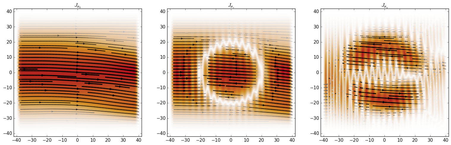
Evaluating a Current operator on a wavefunction returns a
1D array of values that can be directly used with kwant.plotter.current:
Note
Evaluating a Current operator on a wavefunction
returns a 1D array of the same length as the number of hoppings in the
system, ordered in the same way as the edges in the system’s graph.
Similarly to how we saw in the previous section that Density
can be thought of as a collection of operators, Current
can be defined in a similar way. Starting from the definition of a “density”:
we can define currents \(J_{ab}\) via the continuity equation:
where the sum runs over sites \(b\) neigboring site \(a\). Plugging in the definition for \(ρ_a\), along with the Schrödinger equation and the assumption that \(\mathcal{M}\) is time independent, gives:
where latin indices run over sites and greek indices run over the Hilbert space degrees of freedom, and
i.e. \(\mathcal{H}_{ab}\) is a matrix that is zero everywhere except on elements connecting from site \(b\) to site \(a\), where it is equal to the hopping matrix \(\mathbf{H}_{ab}\) between these two sites.
This allows us to identify the rank-4 quantity
as the local current between connected sites.
The diagonal part of this quantity, \(\mathcal{J}_{aa}\),
represents the extent to which the density defined by \(\mathcal{M}_a\)
is not conserved on site \(a\). It can be calculated using
Source, rather than Current, which
only computes the off-diagonal part.
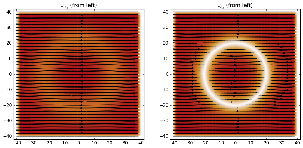
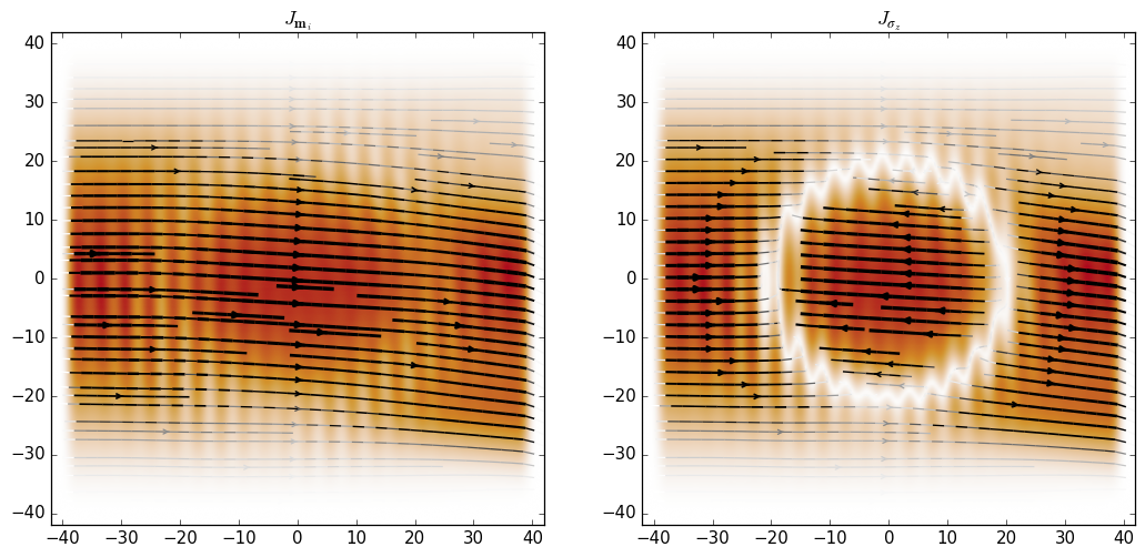
The above examples are reasonably simple in the sense that the book-keeping required to manually calculate the various densities and currents is still manageable. Now we shall look at the case where we wish to calculate some projected spin currents, but where the spin projection axis varies from place to place. More specifically, we want to visualize the spin current along the direction of \(\mathbf{m}_i\), which changes continuously over the whole scattering region.
Doing this is as simple as passing a function when instantiating
the Current, instead of a constant matrix:
    def following_m_i(site, r0, delta):
        m_i = field_direction(site.pos, r0, delta)
        return np.dot(m_i, sigma)

    J_m = kwant.operator.Current(syst, following_m_i)

    # evaluate the operator
    m_current = J_m(psi, params=dict(r0=25, delta=10))
The function must take a Site as its first parameter,
and may optionally take other parameters (i.e. it must have the same
signature as a Hamiltonian onsite function), and must return the square
matrix that defines the operator we wish to calculate.
Note
In the above example we had to pass the extra parameters needed by the
following_operator function via the param keyword argument. In
general you must pass all the parameters needed by the Hamiltonian via
params (as you would when calling smatrix or
wave_function). In the previous examples,
however, we used the fact that the system hoppings do not depend on any
parameters (these are the only Hamiltonian elements required to calculate
currents) to avoid passing the system parameters for the sake of brevity.
Using this we can see that the spin current is essentially oriented along the direction of \(m_i\) in the present regime where the onsite term in the Hamiltonian is dominant:
Another useful feature of kwant.operator is the ability to calculate
operators over selected parts of a system. For example, we may wish to
calculate the total density of states in a certain part
of the system, or the current flowing through a cut in the system.
We can do this selection when creating the operator by using the
keyword parameter where.
To calculate the density of states inside a circle of radius 20 we can simply do:
    def circle(site):
        return np.linalg.norm(site.pos) < 20

    rho_circle = kwant.operator.Density(syst, where=circle, sum=True)

    all_states = np.vstack((wf(0), wf(1)))
    dos_in_circle = sum(rho_circle(p) for p in all_states) / (2 * pi)
    print('density of states in circle:', dos_in_circle)
density of states in circle: 859.766518808
note that we also provide sum=True, which means that evaluating the
operator on a wavefunction will produce a single scalar. This is semantically
equivalent to providing sum=False (the default) and running numpy.sum
on the output.
Below we calculate the probability current and z-projected spin current near the interfaces with the left and right leads.
    def left_cut(site_to, site_from):
        return site_from.pos[0] <= -39 and site_to.pos[0] > -39

    def right_cut(site_to, site_from):
        return site_from.pos[0] < 39 and site_to.pos[0] >= 39

    J_left = kwant.operator.Current(syst, where=left_cut, sum=True)
    J_right = kwant.operator.Current(syst, where=right_cut, sum=True)

    Jz_left = kwant.operator.Current(syst, sigma_z, where=left_cut, sum=True)
    Jz_right = kwant.operator.Current(syst, sigma_z, where=right_cut, sum=True)

    print('J_left:', J_left(psi), ' J_right:', J_right(psi))
    print('Jz_left:', Jz_left(psi), ' Jz_right:', Jz_right(psi))
J_left: 0.979853902635  J_right: 0.979853902635
Jz_left: 0.971465681199  Jz_right: 0.984049935823
We see that the probability current is conserved across the scattering region, but the z-projected spin current is not due to the fact that the Hamiltonian does not commute with \(σ_z\) everywhere in the scattering region.
bind for speed¶In most of the above examples we only used each operator once after creating it. Often one will want to evaluate an operator with many different wavefunctions, for example with all scattering wavefunctions at a certain energy, but with the same set of parameters. In such cases it is best to tell the operator to pre-compute the onsite matrices and any necessary Hamiltonian elements using the given set of parameters, so that this work is not duplicated every time the operator is evaluated.
This can be achieved with bind:
Warning
Take care that you do not use an operator that was bound to a particular set of parameters with wavefunctions calculated with a different set of parameters. This will almost certainly give incorrect results.
    J_m = kwant.operator.Current(syst, following_m_i)
    J_z = kwant.operator.Current(syst, sigma_z)

    J_m_bound = J_m.bind(params=dict(r0=25, delta=10, J=1))
    J_z_bound = J_z.bind(params=dict(r0=25, delta=10, J=1))

    # Sum current local from all scattering states on the left at energy=-1
    wf_left = wf(0)
    J_m_left = sum(J_m_bound(p) for p in wf_left)
    J_z_left = sum(J_z_bound(p) for p in wf_left)