See also
The complete source code of this example can be found in
graphene.py
In the following example, we are going to calculate the conductance through a graphene quantum dot with a p-n junction and two non-collinear leads. In the process, we will touch all of the topics that we have seen in the previous tutorials, but now for the honeycomb lattice. As you will see, everything carries over nicely.
We begin by defining the honeycomb lattice of graphene. This is
in principle already done in kwant.lattice.honeycomb, but we do it
explicitly here to show how to define a new lattice:
graphene = kwant.lattice.general([(1, 0), (sin_30, cos_30)],
                                 [(0, 0), (0, 1 / sqrt(3))])
a, b = graphene.sublattices
The first argument to the general function is the list of
primitive vectors of the lattice; the second one is the coordinates of basis
atoms. The honeycomb lattice has two basis atoms. Each type of basis atom by
itself forms a regular lattice of the same type as well, and those
sublattices are referenced as a and b above.
In the next step we define the shape of the scattering region (circle again)
and add all lattice points using the shape-functionality:
def make_system(r=10, w=2.0, pot=0.1):

    #### Define the scattering region. ####
    # circular scattering region
    def circle(pos):
        x, y = pos
        return x ** 2 + y ** 2 < r ** 2

    syst = kwant.Builder()

    # w: width and pot: potential maximum of the p-n junction
    def potential(site):
        (x, y) = site.pos
        d = y * cos_30 + x * sin_30
        return pot * tanh(d / w)

    syst[graphene.shape(circle, (0, 0))] = potential
As you can see, this works exactly the same for any kind of lattice. We add the onsite energies using a function describing the p-n junction; in contrast to the previous tutorial, the potential value is this time taken from the scope of make_system, since we keep the potential fixed in this example.
As a next step we add the hoppings, making use of
HoppingKind. For illustration purposes we define
the hoppings ourselves instead of using graphene.neighbors():
hoppings = (((0, 0), a, b), ((0, 1), a, b), ((-1, 1), a, b))
The nearest-neighbor model for graphene contains only
hoppings between different basis atoms. For this type of
hoppings, it is not enough to specify relative lattice indices,
but we also need to specify the proper target and source
sublattices. Remember that the format of the hopping specification
is (i,j), target, source. In the previous examples (i.e.
Matrix structure of on-site and hopping elements) target=source=lat, whereas here
we have to specify different sublattices. Furthermore,
note that the directions given by the lattice indices
(1, 0) and (0, 1) are not orthogonal anymore, since they are given with
respect to the two primitive vectors [(1, 0), (sin_30, cos_30)].
Adding the hoppings however still works the same way:
syst[[kwant.builder.HoppingKind(*hopping) for hopping in hoppings]] = -1
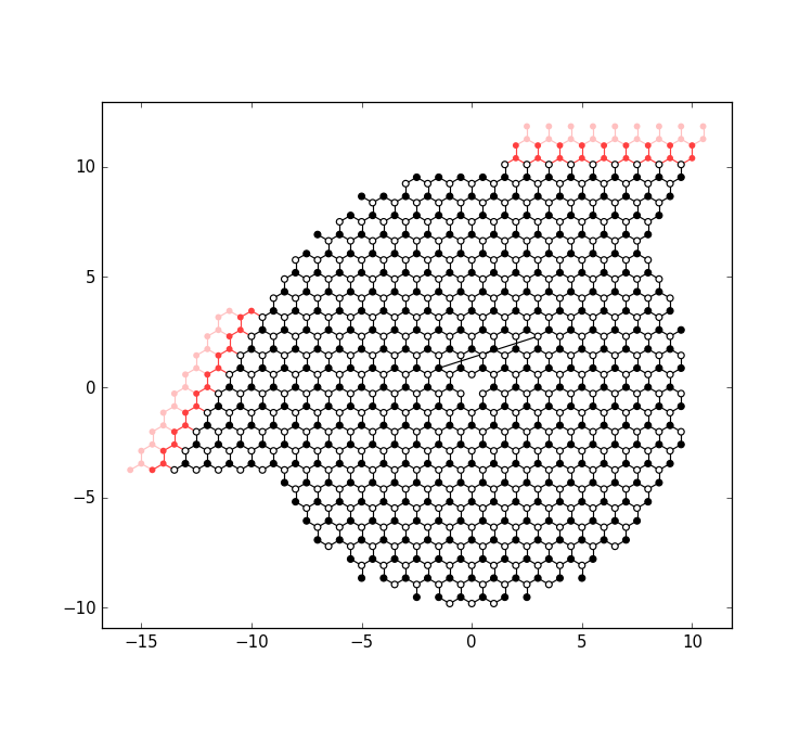
Modifying the scattering region is also possible as before. Let’s do something crazy, and remove an atom in sublattice A (which removes also the hoppings from/to this site) as well as add an additional link:
    del syst[a(0, 0)]
    syst[a(-2, 1), b(2, 2)] = -1
Note again that the conversion from a tuple (i,j) to site is done by the sublattices a and b.
The leads are defined almost as before:
    # left lead
    sym0 = kwant.TranslationalSymmetry(graphene.vec((-1, 0)))

    def lead0_shape(pos):
        x, y = pos
        return (-0.4 * r < y < 0.4 * r)

    lead0 = kwant.Builder(sym0)
    lead0[graphene.shape(lead0_shape, (0, 0))] = -pot
    lead0[[kwant.builder.HoppingKind(*hopping) for hopping in hoppings]] = -1

    # The second lead, going to the top right
    sym1 = kwant.TranslationalSymmetry(graphene.vec((0, 1)))

    def lead1_shape(pos):
        v = pos[1] * sin_30 - pos[0] * cos_30
        return (-0.4 * r < v < 0.4 * r)

    lead1 = kwant.Builder(sym1)
    lead1[graphene.shape(lead1_shape, (0, 0))] = pot
    lead1[[kwant.builder.HoppingKind(*hopping) for hopping in hoppings]] = -1
Note the method vec used in calculating the
parameter for TranslationalSymmetry. The latter expects a
real-space symmetry vector, but for many lattices symmetry vectors are more
easily expressed in the natural coordinate system of the lattice. The
vec-method is thus used to map a lattice vector
to a real-space vector.
Observe also that the translational vectors graphene.vec((-1, 0)) and
graphene.vec((0, 1)) are not orthogonal any more as they would have been
in a square lattice – they follow the non-orthogonal primitive vectors defined
in the beginning.
Later, we will compute some eigenvalues of the closed scattering region without leads. This is why we postpone attaching the leads to the system. Instead, we return the scattering region and the leads separately.
return syst, [lead0, lead1]
The computation of some eigenvalues of the closed system is done in the following piece of code:
def compute_evs(syst):
    # Compute some eigenvalues of the closed system
    sparse_mat = syst.hamiltonian_submatrix(sparse=True)

    evs = sla.eigs(sparse_mat, 2)[0]
    print(evs.real)
Here we use in contrast to the previous example a sparse matrix and the sparse linear algebra functionality of SciPy.
The code for computing the band structure and the conductance is identical to the previous examples, and needs not be further explained here.
Finally, in the main function we make and plot the system:
def main():
pot = 0.1
syst, leads = make_system(pot=pot)
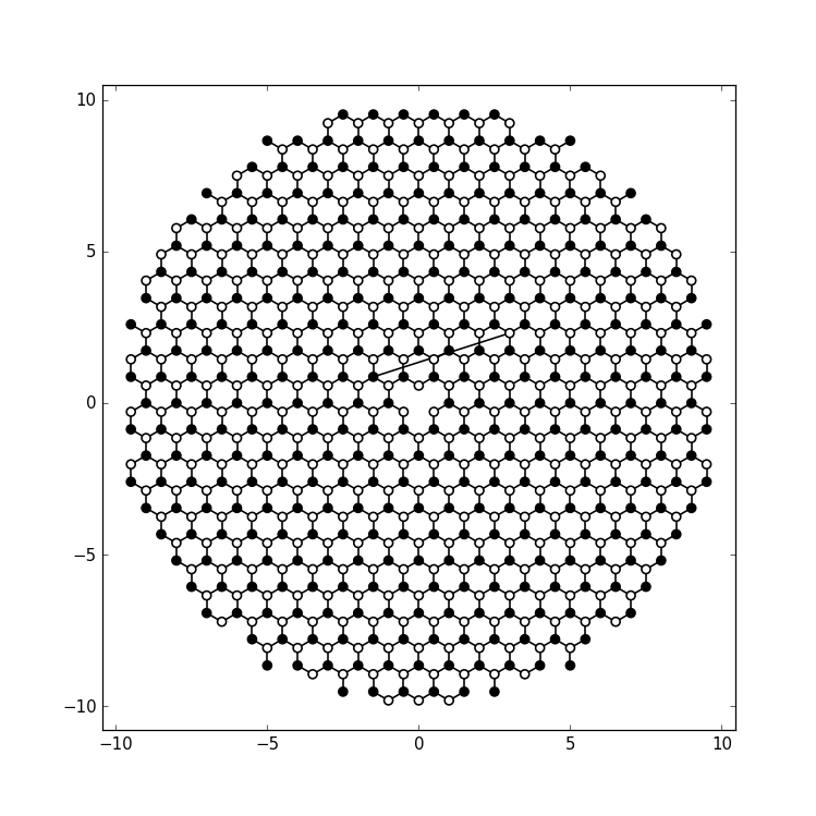
# To highlight the two sublattices of graphene, we plot one with
# a filled, and the other one with an open circle:
def family_colors(site):
return 0 if site.family == a else 1
# Plot the closed system without leads.
kwant.plot(syst, site_color=family_colors, site_lw=0.1, colorbar=False)
We customize the plotting: we set the site_colors argument of
plot to a function which returns 0 for
sublattice a and 1 for sublattice b:
def family_colors(site):
    return 0 if site.family == a else 1
The function plot shows these values using a color scale
(grayscale by default). The symbol size is specified in points, and is
independent on the overall figure size.
Plotting the closed system gives this result:
Computing the eigenvalues of largest magnitude,
compute_evs(syst.finalized())
should yield two eigenvalues equal to [ 3.07869311,
-3.06233144].
The remaining code of main attaches the leads to the system and plots it again:
It computes the band structure of one of lead 0:
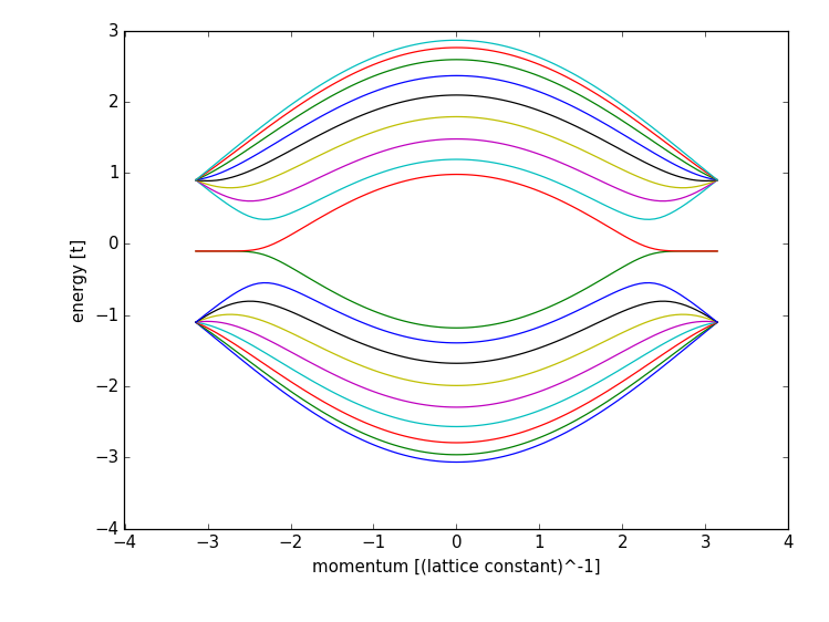
showing all the features of a zigzag lead, including the flat edge state bands (note that the band structure is not symmetric around zero energy, due to a potential in the leads).
Finally the transmission through the system is computed,
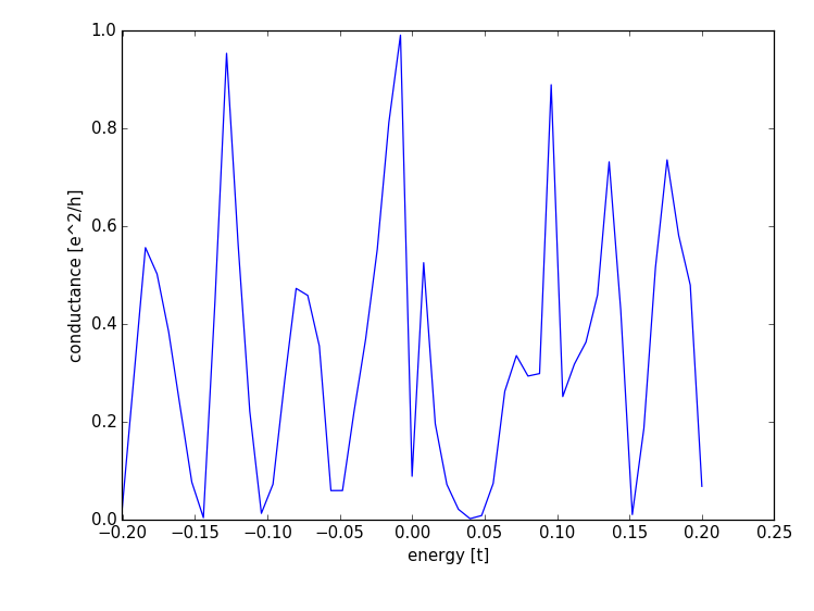
showing the typical resonance-like transmission probability through an open quantum dot
In a lattice with more than one basis atom, you can always act either on all sublattices at the same time, or on a single sublattice only.
For example, you can add lattice points for all sublattices in the current example using:
syst[graphene.shape(...)] = ...
or just for a single sublattice:
syst[a.shape(...)] = ...
and the same of course with b. Also, you can selectively remove points:
del syst[graphene.shape(...)]
del syst[a.shape(...)]
where the first line removes points in both sublattices, whereas the second line removes only points in one sublattice.