This example deals with superconductivity on the level of the Bogoliubov-de Gennes (BdG) equation. In this framework, the Hamiltonian is given as

where  is the Hamiltonian of the system without
superconductivity,
is the Hamiltonian of the system without
superconductivity,  the chemical potential,
  the superconducting order parameter, and
  the time-reversal operator. The BdG Hamiltonian introduces
electron and hole degrees of freedom (an artificial doubling -
be aware of the fact that electron and hole excitations
are related!), which we now implement in Kwant.
the time-reversal operator. The BdG Hamiltonian introduces
electron and hole degrees of freedom (an artificial doubling -
be aware of the fact that electron and hole excitations
are related!), which we now implement in Kwant.
For this we restrict ourselves to a simple spinless system without
magnetic field, so that is just a number (which we
choose real), and  .
.
See also
The complete source code of this example can be found in
tutorial/superconductor_band_structure.py
We begin by computing the band structure of a superconducting wire. The most natural way to implement the BdG Hamiltonian is by using a 2x2 matrix structure for all Hamiltonian matrix elements:
tau_x = tinyarray.array([[0, 1], [1, 0]])
tau_z = tinyarray.array([[1, 0], [0, -1]])


def make_lead(a=1, t=1.0, mu=0.7, Delta=0.1, W=10):
    # Start with an empty lead with a single square lattice
    lat = kwant.lattice.square(a)

    sym_lead = kwant.TranslationalSymmetry((-a, 0))
    lead = kwant.Builder(sym_lead)

    # build up one unit cell of the lead, and add the hoppings
    # to the next unit cell
    for j in xrange(W):
        lead[lat(0, j)] = (4 * t - mu) * tau_z + Delta * tau_x

        if j > 0:
            lead[lat(0, j), lat(0, j - 1)] = -t * tau_z

        lead[lat(1, j), lat(0, j)] = -t * tau_z

    return lead
As you see, the example is syntactically equivalent to our spin example, the only difference is now that the Pauli matrices act in electron-hole space.
Computing the band structure then yields the result
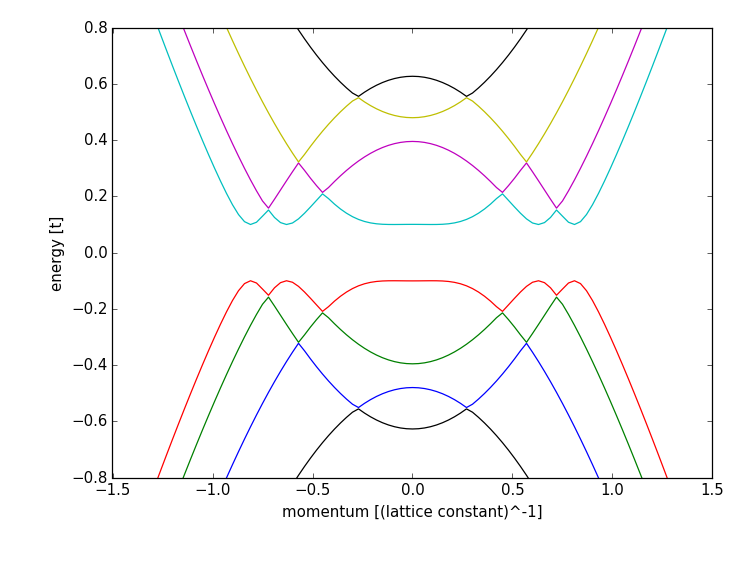
We clearly observe the superconducting gap in the spectrum. That was easy, wasn’t it?
See also
The complete source code of this example can be found in
tutorial/superconductor_transport.py
While it seems most natural to implement the BdG Hamiltonian using a 2x2 matrix structure for the matrix elements of the Hamiltonian, we run into a problem when we want to compute electronic transport in a system consisting of a normal and a superconducting lead: Since electrons and holes carry charge with opposite sign, we need to separate electron and hole degrees of freedom in the scattering matrix. In particular, the conductance of a N-S-junction is given as
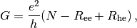
where  is the number of channels in the normal lead, and
 the total probability of reflection from electrons
to electrons in the normal lead, and
the total probability of reflection from electrons
to electrons in the normal lead, and  the total
probability of reflection from electrons to holes in the normal
lead. However, the current version of Kwant does not allow for an easy
and elegant partitioning of the scattering matrix in these two degrees
of freedom [1].
the total
probability of reflection from electrons to holes in the normal
lead. However, the current version of Kwant does not allow for an easy
and elegant partitioning of the scattering matrix in these two degrees
of freedom [1].
In the following, we will circumvent this problem by introducing separate “leads” for electrons and holes, making use of different lattices. The system we consider consists of a normal lead on the left, a superconductor on the right, and a tunnel barrier in between:

As already mentioned above, we begin by introducing two different square lattices representing electron and hole degrees of freedom:
def make_system(a=1, W=10, L=10, barrier=1.5, barrierpos=(3, 4),
                mu=0.4, Delta=0.1, Deltapos=4, t=1.0):
    # Start with an empty tight-binding system and two square lattices,
    # corresponding to electron and hole degree of freedom
    lat_e = kwant.lattice.square(a, name='e')
    lat_h = kwant.lattice.square(a, name='h')
Note that since these two lattices have identical spatial parameters, the
argument name to square has to be different.
Any diagonal entry (kinetic energy, potentials, ...) in the BdG
Hamiltonian corresponds to on-site energies or hoppings within
the same lattice, whereas any off-diagonal entry (essentially, the
superconducting order parameter ) corresponds
to a hopping between different lattices:
    sys = kwant.Builder()

    #### Define the scattering region. ####
    sys[(lat_e(x, y) for x in range(L) for y in range(W))] = 4 * t - mu
    sys[(lat_h(x, y) for x in range(L) for y in range(W))] = mu - 4 * t

    # the tunnel barrier
    sys[(lat_e(x, y) for x in range(barrierpos[0], barrierpos[1])
         for y in range(W))] = 4 * t + barrier - mu
    sys[(lat_h(x, y) for x in range(barrierpos[0], barrierpos[1])
         for y in range(W))] = mu - 4 * t - barrier

    # hoppings for both electrons and holes
    sys[lat_e.neighbors()] = -t
    sys[lat_h.neighbors()] = t

    # Superconducting order parameter enters as hopping between
    # electrons and holes
    sys[((lat_e(x, y), lat_h(x, y)) for x in range(Deltapos, L)
         for y in range(W))] = Delta
Note that the tunnel barrier is added by overwriting previously set on-site matrix elements.
Note further, that in the code above, the superconducting order parameter is nonzero only in a part of the scattering region. Consequently, we have added hoppings between electron and hole lattices only in this region, they remain uncoupled in the normal part. We use this fact to attach purely electron and hole leads (comprised of only electron or hole lattices) to the system:
    # Symmetry for the left leads.
    sym_left = kwant.TranslationalSymmetry((-a, 0))

    # left electron lead
    lead0 = kwant.Builder(sym_left)
    lead0[(lat_e(0, j) for j in xrange(W))] = 4 * t - mu
    lead0[lat_e.neighbors()] = -t

    # left hole lead
    lead1 = kwant.Builder(sym_left)
    lead1[(lat_h(0, j) for j in xrange(W))] = mu - 4 * t
    lead1[lat_h.neighbors()] = t
This separation into two different leads allows us then later to compute the reflection probablities between electrons and holes explicitely.
On the superconducting side, we cannot do this separation, and can only define a single lead coupling electrons and holes (The += operator adds all the sites and hoppings present in one builder to another):
    sym_right = kwant.TranslationalSymmetry((a, 0))
    lead2 = kwant.Builder(sym_right)
    lead2 += lead0
    lead2 += lead1
    lead2[((lat_e(0, j), lat_h(0, j)) for j in xrange(W))] = Delta
We now have on the left side two leads that are sitting in the same spatial position, but in different lattice spaces. This ensures that we can still attach all leads as before:
    sys.attach_lead(lead0)
    sys.attach_lead(lead1)
    sys.attach_lead(lead2)

    return sys
When computing the conductance, we can now extract reflection from
electrons to electrons as smatrix.transmission(0, 0) (Don’t get
confused by the fact that it says transmission – transmission
into the same lead is reflection), and reflection from electrons to holes
as smatrix.transmission(1, 0), by virtue of our electron and hole leads:
def plot_conductance(sys, energies):
    # Compute conductance
    data = []
    for energy in energies:
        smatrix = kwant.smatrix(sys, energy)
        # Conductance is N - R_ee + R_he
        data.append(smatrix.submatrix(0, 0).shape[0] -
                    smatrix.transmission(0, 0) +
                    smatrix.transmission(1, 0))
Note that smatrix.submatrix(0,0) returns the block concerning reflection
within (electron) lead 0, and from its size we can extract the number of modes
.
Finally, for the default parameters, we obtain the following result:
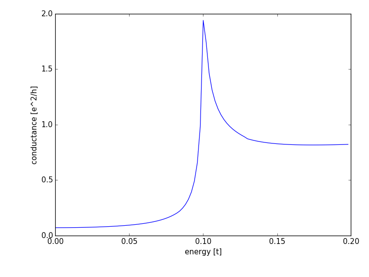
We a see a conductance that is proportional to the square of the tunneling probability within the gap, and proportional to the tunneling probability above the gap. At the gap edge, we observe a resonant Andreev reflection.
smatrix returns an array containing
the transverse wave functions of the lead modes (in
SMatrix.lead_info.
By inspecting the wave functions, electron and hole wave
functions can be distinguished (they only have entries in either
the electron part or the hole part. If you encounter modes
with entries in both parts, you hit a very unlikely situation in
which the standard procedure to compute the modes gave you a
superposition of electron and hole modes. That is still OK for
computing particle current, but not for electrical current).Footnotes
| [1] | Well, there is a not so elegant way to do it still. See the technical details |